
A Composite Indicators Approach to Assisting Decisions in Ship
LCA/LCC
Yiannis Smirlis
1a
and Marc Bonazountas
2
1
School of Economics, Business and International Studies, University of Piraeus, Greece
2
EPSILON Malta, Ltd, Tower Business Center, Swatar, Malta
Keywords: Ship, Life Cycle Assessment, Key Performance Indicators-KPIs, Composite Indicators.
Abstract: During of the life cycle of ship, multiple decisions concerning design, operation and demolition must be made.
The Life Cycle Assessment/Cost (LCA/LCC) framework applied in ships, mandates that such decisions need
to encounter dominant economic and environmental aspects about the ship. In this paper we consider these
decisions in the context of Multi-Criteria Decision Analysis and present a methodology to construct composite
indicators to assist decision making. For the criteria introduced we propose the use of key performance
indicators (KPIs) that quantify economic and environmental dimensions. For the construction, aggregation
and weighting of the KPIs we present linear programming models that estimate the weights endogenously
from the data. The models developed can discriminate the optimum designs, thus assisting decision making.
1 INTRODUCTION
A ship Life Cycle Assessment (LCA) is a framework
to evaluating different economic and environmental
aspects and impacts, from its design and building
from raw materials, through operation, maintenance,
end-of-life treatment, recycling and final disposal to
its end of lifetime. It is a tool to better understand
costs, risks, opportunities, trade-offs and nature of
environmental impacts. LCA can assist in identifying
opportunities to improve the environmental
performance of a ship at various points in its life
cycle, in informing decision and policy makers in the
maritime industry and in selecting relevant indicators
of economic and environmental performance.
The basic theory of LCA (Curran, 1996) is
transferred to the field of maritime and shipping from
the products and services design throughout their
lifespan. For the products, the requirements and the
implementing guidelines for LCA is covered by the
international standards ISO 14040 and 14044 (ISO
2006). Especially the economic impact of LCA, has
been addressed by the concept of Life Cycle Cost
(LCC) (Aurich et. al., 2007; Dhillon, 2013). LCC
aims to identify factors that affect cost, to quantify
them and to evaluate the cost effectiveness of
a
https://orcid.org/0000-0002-6608-3326
alternative strategies to incur over a specified period
of time. LCA/LCC were applied to energy systems,
electromobility, buildings and built environment,
food and agriculture, biofuels and biomaterials,
chemicals, wastewater treatment, solid waste
management, etc. (Hauschild et. al, 2018).
Ships, seen as complex systems, integrated in
economic, technical and transportation activities,
need to be studied in line with the concept of
LCA/LCC (Marius, 2014; Angelfoss, 1998). Ships’
life cycle is decomposed in three phases: the design
and ship building (phase I), the operation &
maintenance (phase II), and the end-of-life,
demolition and disposal (phase III). During the ships’
life, designers, shipowners, executives, and others,
are confronted with different decision situations that
are complex and involve a large number of options
and alternatives. For example, in the ship
design/construction phase, shipbuilders -- based on a
primitive ship construction (ship reference) that
fulfils all the technical, cruising, safety and
environmental regulations -- have a large number of
options to consider and evaluate as type of fuel and
engines, materials for the structure and
superstructure, type of generators. Every single
combination, if applied to the final ship structure, has
economic and environmental consequences.
Smirlis, Y. and Bonazountas, M.
A Composite Indicators Approach to Assisting Decisions in Ship LCA/LCC.
DOI: 10.5220/0008895401430150
In Proceedings of the 9th International Conference on Operations Research and Enterprise Systems (ICORES 2020), pages 143-150
ISBN: 978-989-758-396-4; ISSN: 2184-4372
Copyright
c
2022 by SCITEPRESS – Science and Technology Publications, Lda. All rights reserved
143

During the operation phase of a ship, the
LCA/LCC approach may give useful answers to
questions such as which technical adjustments are
cost /environmental effective so to reduce operating
expenses? which are the most beneficial options for
ship lay-up or hire out for offshore storage facility?
which is the most environmental friendly and cost
efficient solution among alternatives such as to burn
diesel fuel inside ECA or to install scrubbing
technology or even after a costly damage? which
alternative decisions (in terms of costs) are the most
valuable: repair the vessel? to sell the ship in the
second-hand market or to sell ship for scrap?. Finally,
in the end-of-life period, the decision whether to
dismantle a ship or continue the activity by
restructuring it in a retrofit procedure or convert it to
another type of maritime mission, requires both
technical condition assessment and economic
evaluation since a decision may end up in adverse
economic results, with a negative impact on the
environment.
In this paper we allege that a significant number
of problems that arise during the life cycle of a ship
with the context of LCA/LCC, can be formulated and
considered under the scope of decision-making
theory. Accordingly, a decision-maker is called to
evaluate alternatives on the basis of two or more
criteria so to discriminate the superior in terms of
economy and environmental impact. For the criteria,
we particularly consider established economic and
environmental key performance indicators (KPIs)
that measure the performance of each alternative
decision in specific aspects (ship building cost,
operational expenses, maintenance and repair costs,
energy efficiency, NOx/Sox emissions etc.). Then,
based on mathematical programming methods, we
propose to aggregate the KPIs in composite indicators
that express more abstract concepts, understandable
by the users thus assisting the decision-making
process.
This paper is organized as follows. Section 2
presents the relation of KPIs used as criteria in the
decision-making LCA processes. Section 3 presents
the construction of composite indicators so to exploit
KPIs and assist decision making by identifying the
optimized alternative decisions. Section 4 presents an
illustrative example for evaluating alternative ship
designs. Conclusions appear at the end of this paper.
2 KPIs AND COMPOSITE
INDICATORS IN SHIP LIFE
CYCLE ASSESSMENT
Key performance indicators (KPIs) within the
LCA/LCC framework are quantifiable performance
measurements used for specific economic, technical,
operational and environmental dimensions of a ship.
Common KPIs, potentially used in ship LCA/LCC
are the: (1) Building Cost, Capital Expenditure
(CAPEX), (2) Operational Expenditure (OPEX), (3)
Maintenance and Repair costs (MRC), (4) Average
Annual Cost (AAC), (5) Required Freight Rate
(RFR), (6) Net Present Value (NPV), (7) Average
Annual Benefits (AAB), (8) Earnings Before
Interests, Taxes, Depreciation and Amortization
(EBITDA), (9) Return on Investment Capital (ROIC),
and (10) Energy Efficiency Design Index (EEDI).
KPIs like the above, are provided in different units,
dollars, number of years etc., may have any scale of
measurement, ratio, ordinal etc. and may have
positive contribution/utility (e.g., NPV, EBITDA,
EEDI) or negative (OPEX, MRC, AAC, NOx/Sox
emissions). Such KPIs have been used in past
research studies to estimate the ships’ performance.
For instance, the work of Gratsos & Zachariadis
(2009) examines the importance of the Average
Annual Cost (AAC) as an indicator to evaluating
different ship designs that technically appear as
optimized. Furthermore, the Energy Efficiency of
Operation (EEO) (Lu et al., 2015) is defined and
utilized to predict the operational ship performance.
According to the LCA/LCC, KPIs are used for
measuring costs, revenues, energy efficiency, etc., not
only for a specific period but for the entire lifecycle
of the ship. For example, during the ship design (first
phase of LCA), different ship models and
configurations are evaluated in terms of operating –
maintenance costs, total revenues gained during the
operation phase, price at the time of demolition,
potential use of recycled materials etc. In this context,
the decision-making problem is to identify those
alternative designs that have the total optimum
performance (minimum costs, maximum revenues,
minimum environmental impact). This goal cannot be
achieved by only exploiting KPIs, because they are of
low-level and measure only partial dimensions.
Furthermore, KPIs may usually conflict one another.
For example, a ship built with low budget, at the
operation stage may have higher maintenance and
repair costs.
ICORES 2020 - 9th International Conference on Operations Research and Enterprise Systems
144
In this study we propose as more beneficial for the
assessment of different alternative decisions the use
of composite indicators derived from the aggregation
of properly selected KPIs. Composite indicators, in
general, are commonly used for benchmarking of
entities, summarizing in a single measurement,
complex social, economic, environmental etc.
concepts by involving several thematically related
sub-indicators. According to our approach, composite
indicators’ that measure abstract concepts such as
“economic benefits”, “environmental impact” etc.,
meaningful to a decision-maker, may derive from the
aggregation of the values of individual sub-indicators
(KPIs).
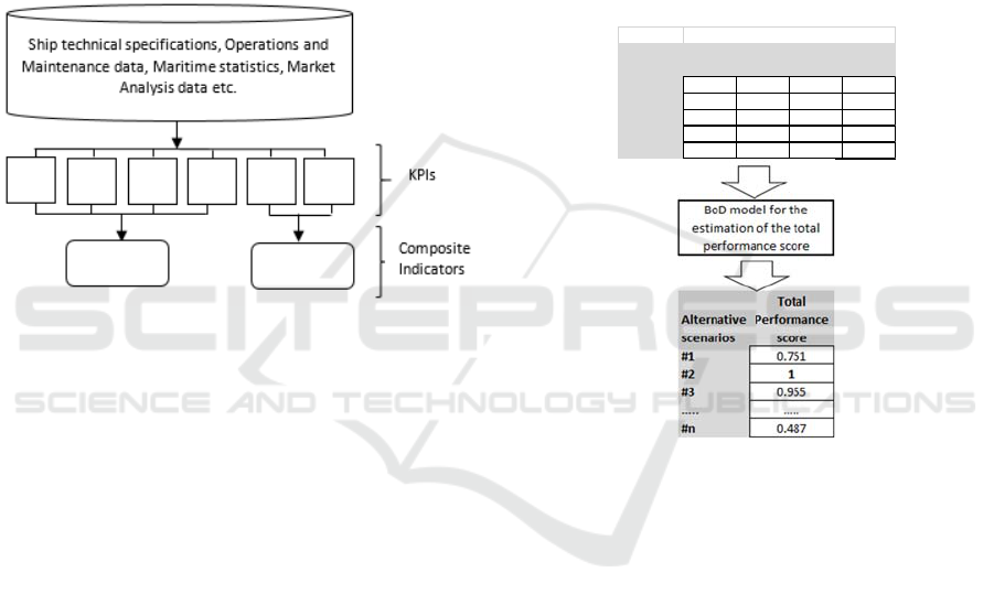
Figure 1: The hierarchy of data processing, from raw data
to KPIs and composite indicators.
Figure 1 presents the place of the composite
indicators in the hierarchy of data processing,
deriving from KPIs regarded as sub-indicators which
in turn are estimated from data sources (ship technical
specifications, Operations and Maintenance data,
Maritime statistics, Market Analysis data etc.).
3 DERIVATION OF THE
COMPOSITE INDICATORS
In the derivation process of composite indicators, the
aggregation and the weighting are the most important
steps and for them, a number of alternative
methodologies (Nardo et al. 2005, OECD 2008) have
been proposed to substitute the common approach of
using additive or multiplicative average formulas in
conjunction with constant, predetermined values for
the weights: Principal components/Factor analysis,
Benefit of the doubt approach, Unobserved
components model, Budget allocation process,
Analytic hierarchy process, Conjoint analysis etc.
Among them, the Benefit of the doubt (BoD)
modelling (Melyn and Moesen, 1991; Cherchye,
2007) uses linear programming and an additive
weighted-based form to estimate the scores of the
composite indicator. Advantage of the method is that
it arranges so the weights of the sub-indicators to
derive directly from that data, endogenously, as result
of an optimization process. BoD is inspired by the
multiplier formulation of Data Envelopment Analysis
(DEA) (Charnes et. al, 1978) as it estimates different
weights for each unit (alternative design) under
assessment, choosing the most favourable values so
to let them reach the highest possible score. BoD
modelling can discriminate alternative decisions to
superior and non-superior. Figure 2 depicts the
estimation process.
Figure 2: The estimation of the superiority index from the
decision matrix.
BoD linear programming models are applied to
the decision matrix composed of alternative decision
scenarios and the KPIs (criteria) to obtain a total
performance score. Alternative decisions with score
equal to 1 are regarded as superior. The mathematical
background of this method is briefly described in the
following sub-sections.
3.1 Optimization Models for the
Aggregation and the Weighting of
KPIs
Assume that in a typical assessment in the ship design
/building phase I, n alternative designs have to be
assessed in terms of m KPIs so to derive scores of a
composite indicator. The decision matrix of the
problem is composed of a set of n alternative designs
12
{ , ,..., }
n
Aaa a
and of m individual KPIs
Alternat ive
scenarios KPI_1 KPI_2 ….. KPI_m
#1 0.25 125
0
….. 55.3
#2 0.48 175
0
….. 48.18
#3 1.32 195
0
….. 23.45
….. ….. ….. ….. …..
#n 0.99 980 ….. 60.15
KPIs
A Composite Indicators Approach to Assisting Decisions in Ship LCA/LCC
145

12
, ,...,
m
XX X
,
12
( , ,..., )
iii in
Xxx x
1, ..,im
. The values
, 1,.., , 1,..,
ij
x
imjn
denote the performance score of the alternatives
j
a
on the KPIs
i
X
.For any alternative
j
a
, the
contribution of a the i-th KPI to the total value of the
composite indicator, is expressed by the factor
iij
wx
, with the weight
i
w
to be unknown, under
estimation. In such a setting, the value of the
composite indicator for an alternative
j
derive by the
additive linear form
1
m
j
iij
i
Iwx
. The value
j
I
expresses the total performance of the alternative
j
a
on all the involved KPIs. Consequently if for two
alternatives
12
,
jj
holds
12
j
j
II
, the conclusion is
that alternative
1
j
, is superior (has better
performance) than alternative
2
j
. It is important to
note that this additive form function designates a
compensatory approach (OECD 2008, Bandura 2011)
according to which, any possible disadvantage (low
value) of a particular alternative design in a specific
KPI can be counterbalanced by the advantage (high
value) in other KPIs.
For the estimation of the values of the weights
i
w
, the BoD model (1) is proposed.
00
1
I
m
jiij
i
M
ax w x
1
1, 1, ..,
m
jiij
i
Iwxjn
,1,..,
i
wi m
(1)
Model (1) is solved
n times, once for each alternative
design
0
j
and estimates the optimal values
*
, 1,...,
i
wi m
of the weights so to maximize its
total performance score. Let this score be
0
*
j
I
. The
constraints
1
1, 1, ..,
m
iij
i
wx j n
ensure a
comparative assessment and set maximum attainable
score
0
*
j
I
equal to 1. The factor ε in the constraint
,1,..,
i
wi m
, seen as a parameter, is assigned
small values (approximately ε =10
-6
) and prevents the
weights to accept zero values. Model (1) is able to
discriminate alternative designs to superior and non-
superior. Superior are those that, in the comparative
process, achieved to reach the upper bound score 1 by
selecting the proper optimal values
*
i
w
(superior
alternatives={
*
:1
j
jI
}) and non-superior are
those that did not succeeded to do so ( non-Superior
alternatives ={
*
:1
j
jI
}).
About the meaning of the weights
i
w
and the
values that can be assigned to them, it is necessary to
point out that they must not be considered as
importance coefficients that reflect the contribution
of a KPI to the value
*
j
I
but rather as the “trade-off”
factors expressing the marginal rate of substitution
between two alternatives (Decancq and Lugo 2013).
In sub-section 3.4 the issue of restricting them
according to the users’ opinion will be discussed.
Despite the flexibility of Model (1) to choose the
weight values directly from the data, there are certain
drawbacks: it provides unrealistic weight values, it
privileges the alternatives with high performance to
only few sub-indicators, it is not capable to
discriminate those that achieve the highest score 1
and due to different set of weights, lacks a common
cross-alternative comparison (Zhou et al. 2007). The
latter can be resolved by a model variation that uses
common set of weight values. The issue of common
weights in BoD has been transferred again from the
similar DEA context (see Kao (2010), Bernini et al.
(2013), Koronakos et al (2019)). The modified
extension of model (1) with common weights is
formulated as follows.
For an alternative
j, let
j
d
be the difference
between the sum
1
m
iij
i
wx
and the 1 (the deviation
factor from the absolute attainable score 1), i.e.
1
1
m
j
iij
i
dwx
. By its definition,
j
d
is a positive
number
0
j
d
, while the sum
1
n
j
j
d
denotes the
total deviation of all the alternatives from the absolute
score 1. The basic idea behind the common
assessment is to let alternatives cooperate in order to
get as close as possible to the absolute score 1. This
approach can be characterized as fair and democratic
since all the alternatives, collectively and equally,
participate to the generation of the optimal set of
common weights that yield the composite index. In
terms of linear programming, this is translated as a
goal to minimize the total deviation expressed by the
ICORES 2020 - 9th International Conference on Operations Research and Enterprise Systems
146

sum
1
n
j
j
d
. Model (2) achieves to do so.
1
n
j
j
M
in d
1
1, 1, ..,
m
iij j
i
wx d j n
,1,..,
0, 1,..,
i
j
wi m
djn
(2)
In model (2), the objective function minimizes the
sum of the deviations (distance of
L
1
norm) of all
alternatives between the performance that they can
achieve using the common multipliers and their ideal
rating. Compared to model (1), model (2) requires
less computational effort as it is solved only once and
it produces lower scores from model (1), thus
providing higher discrimination.
3.2 Controlling the Number of
Superior Alternatives
About the parameter ε, it is important to notice that
higher values than ε =10-6 reduce the number of
superior alternatives and thus affect the
discriminating power of the method (Cook et al.
1996). Large enough values may result to infeasibility
of model (1). The greatest unique value of ε, say ε*
that makes model (1) feasible, ensures that only one
superior, the best, alternative is obtained from the
process (Toloo & Tavana 2016). Such a value ε* can
be estimated by model (1) when its objective function
is replaced by
ε
M
ax
and the rest of the constraints
remain unchanged.
3.3 Normalization
Models (1)-(2) are capable to incorporate data from
KPIs that are expressed in different measurement
units (dollars, years of ship operation, etc.). However,
normalization of the data in KPIs is needed before
applying the aggregation step. The main reason is to
convert the data so all KPIs to have a positive
contribution or utility – higher values are more
desirable (for example Operational Expenditure -
OPEX). Another reason is that models (1)-(2) are
sensitive to outliers and to highly skewed data. The
normalization can be achieved with different
methodologies for example min-max, z-score etc.
3.4 Implementation of
Decision-Makers’ Preferences
Models (1)-(2) give freedom to the alternative designs
to assign such weight values so to appear as superior
as possible. This means that any design can appear as
excellent performer by overestimating those KPIs
that has advantage over the rest. However, this
situation may give results that contradict to prior
common views and overestimate KPIs that are
insignificant to the decision-maker. Fortunately, BoD
models are able to incorporate prior information by
imposing additional weight restrictions that express
the common value judgments of the decision maker.
The most important are those of type “pie-share”,
initially proposed by Wong and Beasley (1990) and
classified by Cherchye et al. (2007), that affect the
contribution of each KPI to the total indicator score.
For example the constraint
1
iij
m
iij
i
wx
ab
wx
,
imposes that the proportion /share of the i-th KPI will
vary between the constants
,ab
. In the same manner,
ordinal constraints of the “share” type can be adopted
to prioritize the contribution of a KPI over others.
This type of restrictions overcome the difficulty on
the interpretation of the weights and shift the focus to
KPI shares which are completely independent of
measurement units and easily understandable by the
decision makers.
4 ILLUSTRATIVE EXAMPLE
Assume that in the design /building phase of a new
40,000 DWT (Handymax) bulk carrier ship, the basic
technical specifications have been decided so to
consist the basic ship reference. Based on that, 18
alternative designs are considered as feasible for
implementation. These derive as distinct
combinations of different types of superstructure
materials (steel of various strength), of engines (2-4
strokes DE, Gas turbine etc) and equipment
(scrubber, ballast water treatment system, etc). The
problem under consideration is, which set of the
alternative designs achieve the best performance in
terms of economy and environmental impact,
considering the whole life of the ship, from its first
day of operation to its last. The proposed approach of
this paper is to define two composite indicators, say
ECO for economy and ENV for the environment,
estimate their values for all the alternative designs
A Composite Indicators Approach to Assisting Decisions in Ship LCA/LCC
147

and by comparing them, identify the most optimised
designs, the ones candidate for implementation.
For this problem, a number of KPIs may be
selected to describe both the economic and
environmental dimensions. In this example, we
further assume that a decision maker selects as the
most appropriate for the ship economy three KPIs,
namely the CAPEX, OPEX to represent costs and
AAB for the revenues. CAPEX measures, in thousand
$, the funds that a ship owner uses to purchase a
vessel from a shipyard, OPEX accounts in thousand $
per year, the ongoing costs that a ship owner pays to
run the ship over a specific period, e.g. typical year of
operation, while AAB represents the revenues and is
the average annual benefits form the ship, measured
in thousand $ per year. The details (formulas, data
parameters) for the estimation of these KPIs are not
mentioned here due to the limited size of the paper.
Accordingly, the environmental savings are described
by EEDI (Energy Efficiency Design Index) and the
NOx and Sox emissions calculated from the technical
specifications of each alternative design.
The values of the above mentioned KPIs appear
in Table 1. In this table, the first design, indicated as
REF, corresponds to the basic ship reference that
participates in the assessment equally with the rest of
the alternative designs.
Table 1: The basic data set.
Desgin CAPEX OPEX AAB EEDI NOx SOx
REF 6582 1.454 5.836 6.8 13.81 3.45
d1 5377.1 1.447 3.494 7.7 12.3 2.26
d2 5751.8 1.507 3.613 3.6 11.46 1.25
d3 5924.2 1.362 5.284 4.5 11.99 2.92
d4 6914.8 1.61 3.856 4.2 11.14 1.96
d5 5432.2 1.328 5.397 4 12.09 3.74
d6 5754.8 1.567 4.728 3.9 14.37 1.98
d7 5650.4 1.6 6.023 3.1 11.01 1.5
d8 5524.8 1.362 3.863 2.9 12.9 2.21
d9 6718.6 1.61 3.8 4 12.09 3.74
d10 7180.9 1.328 3.893 4.4 11.39 1.81
d11 5944.9 1.424 3.875 5.6 14.44 3.75
d12 7056.5 1.575 4.388 4 12.09 3.74
d13 5360.7 1.338 5.879 3.2 11.35 4.98
d14 5412.5 1.297 4.691 6.8 13.99 2.48
d15 6247.4 1.547 3.474 7.7 11.66 3.76
d16 6526.3 1.61 5.157 4 12.09 3.74
d17 5337.8 1.328 4.058 3.4 12.51 2.6
d18 6260.3 1.435 5.165 7.9 11.03 4.43
From inspecting the data in Table 1, we may
notice that a number of alternatives (e.g. d2) have
adequate performance on economy and poor in the
environmental KPIs while for others (e.g. d14) is
vice-versa.
In order to estimate the values of the composite
indicators ECO, ENV, models (1), (2) are applied to
the data set. Before that, a normalization process (see
Section 3.3) eliminates the differences in the scales of
measurement and reverses to positive the values for
the indicators with negative utility such as CAPEX,
OPEX, NOx, SOx. In such an arrangement the two
composite indicators ECO, ENV appear both with
positive utility (the higher the values, the better is the
design). Moreover, for the estimation of the economy
indicator ECO, we considered as most important the
AAB sub-indicator, giving emphasis to the revenues.
Accordingly, for the ENV indicator, the most
important sub-indicator is considered EEDI. This
initial information is implemented to the modelling as
ordinal weight restrictions of type “share” (see
Section 3.2). The values resulted from the model
application for the composite indicators ECO and
ENV, appear in the last four columns of Table 1.
The values of composite indicators ECO, ENV
derived from models (1)-(2) appear in Table 2.
Table 2: The values of the two composite indicators ECO,
ENV obtained by Models (1), (2).
Model (1) Model (2)
Design ECO ENV ECO ENV
REF 0.949 0.708 0.935 0.644
d1 0.796 0.766 0.806 0.797
d2 0.784 0.935 0.788 0.802
d3 0.934 0.858 0.941 0.747
d4 0.747 0.923 0.757 0.894
d5 0.969 0.875 0.970 0.695
d6 0.863 0.788 0.844 0.763
d7 1.000 1.000 0.923 1.000
d8 0.840 1.000 0.855 0.780
d9 0.749 0.875 0.756 0.695
d10 0.791 0.898 0.842 0.908
d11 0.813 0.708 0.827 0.609
d12 0.790 0.875 0.799 0.695
d13 1.000 0.970 1.000 0.687
d14 0.928 0.700 0.936 0.710
d15 0.747 0.802 0.758 0.713
d16 0.863 0.875 0.848 0.695
d17 0.873 0.902 0.885 0.752
d18 0.898 0.839 0.902 0.719
Based on the results presented in Table 2, a
number of remarks are possible. First, focusing on the
results of model (1), several designs appear as
superior (score equal to 1) in one of the two
dimensions. This is the case for designs d7 and d13
on economy (ECO indicator) and d7 and d8 on the
environment (ENV indicator). Only design d7 is the
best in both economics and environment and
presumably this design is suggested as the optimum
that achieves reduction of costs and the best
environmental protection. Scores obtained from
model (2) with common weights are lower that those
from model (1). Consequently, alternative d8 loses its
ICORES 2020 - 9th International Conference on Operations Research and Enterprise Systems
148
superiority classification and only d7 and d13 are
superior in ENV and ECO, respectively. Note that in
this model, no alternatives are optimum in both
composite indicators.
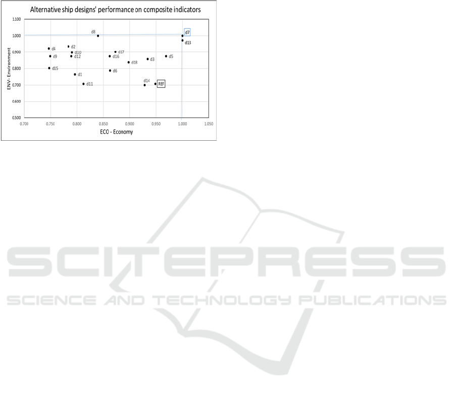
Figure 3: Graph of the values ENV, ECO composite
indicators derived from models (1)-(2).
Figure 3 presents the scores of designs in two axes
ENV and ECO, as obtained from model (1). Design
d7 located at the upper right corner with score 1 on
both ECO, ENV indicators is the best alternative.
Other alternatives that lie on the horizontal and
vertical boundaries (score 1) are superior in only one
dimension. Note that the basic reference design
(REF), being in an intermediate position, did not
achieved to reach superiority as other designs have
been proved better than this.
5 CONCLUSIONS
This study contributes to the ship LCA/LCC concept
by suggesting composite indicators to assist decision
making. Decision situations are formulated as multi-
criteria decision making/analysis problems in which,
key performance indicators-KPIs are considered as
economic and environmental criteria while the
different decisions to be made consists the
alternatives. The composite indicators use simple,
additive weighting sum to aggregate the KPIs so to
obtain scores for the alternative decisions. The
aggregation and the weighting of the KPIs is based to
linear programming models and the weights are
estimated endogenously from the data. The proposed
models are able to reveals the optimum performance
alternatives, those that minimize costs, maximize
revenues and minimize environmental impact.
The proposed methodology is simple to use and
implement without needing the user interaction. It is
flexible to accept initial information as user
preferences in order to access alternatives by a specific
priority on KPIs. Furthermore, the modelling presented
can be easily expanded to cover cases when the KPIs
are expressed in ordinal form or include uncertainty,
being expressed with intervals with constant bounds.
We hope you find the information in this template
useful in the preparation of your submission.
ACKNOWLEDGEMENTS
This study was co-funded by the European Maritime
and Fisheries Fund (EMFF) programme of the
European Union under Grant Agreement No 863565.
The EU support has been appreciated.
REFERENCES
Allen, R., Athanassopoulos A., Dyson R. G., Thanassoulis
E., 1997. Weights restrictions and value judgments in
Data Envelopment Analysis: Evolution, development
and future directions. Annals of Operations Research
73 0: 13-34 doi: 10.1023/A:1018968909638
Angelfoss, A. 1998. Life Cycle Evaluations of Ship
Transportation, Workshop April 15.-16., Ålesund
College, Report no. 10/B101/R-98/004/00, 1998.
Aurich, C., Schweitzer E., and Fuchs C. 2007. Life cycle
management of industrial product-service systems.
Advances in Life Cycle Engineering for Sustainable
Manufacturing Businesses. Springer London, 171-176.
Bandura, R., 2011. Composite indicators and rankings:
Inventory 2011. Technical report, Office of
Development Studies, United Nations Development
Programme (UNDP), New York.
Bernini, C., Guizzardi, A., Angelini, G., 2013. DEA-like
model and common weights approach for the
construction of a subjective community well-being
indicator. Social Indicators Research, 114(2), 405–424.
Charnes, A., Cooper, W. and Rhodes, E., 1978. Measuring
the efficiency of decision making units. European
Journal of Operational Research 2: 429-444.
Cherchye, L, Moesen, W., Rogge, N. and Van
Puyenbroeckan, T. 2007. Introduction to ‘Benefit of the
Doubt’ composite indicators, Social Indicators Research
82: 111–145 doi: 10.1007/s11205-006-9029-7
Cook, W. D., Kress, M., Seiford, L. M. 1996. Data
envelopment analysis in the presence of both
quantitative and qualitative factors. Journal of
Operational Research Society, 47, 945–953.
Curran, M. A., 1996. Environmental life-cycle assessment.
The International Journal of Life Cycle Assessment,
Volume 1, Issue 3, 1996.
Decancq, K., Lugo, M. A., 2013. Weights in
multidimensional indices of wellbeing: An overview.
Econometric Reviews, 32(1), 7–34.
Dhillon, B., 2013. Life cycle costing: techniques, models and
applications, Routledge ed. ISBN: 978-2881243028
A Composite Indicators Approach to Assisting Decisions in Ship LCA/LCC
149

Gratsos, G, Zachariadis, P., 2009. Life cycle cost of
maintaining the effectiveness of a ship’s structure and
environmental impact of ship design parameters.
Helenic Chamber of Shipping. Available at
http://nee.gr/downloads/60Life.cycle1.pdf
Hauschild, M., Rosenbaum, R., Olsen, S., 2018. Life Cycle
Assessment: Theory and Practice, Springer ed. ISBN
978-3-319-56474-6.
ISO, 2006. https://iso.org/standard/37456.html,
https://iso.org/standard/72357.html
Kao, C., 2010. Weight determination for consistently
ranking alternatives in multiple criteria decision
analysis. Applied Mathematical Modelling, 34(7),
1779–1787.
Koronakos, G., Smirlis, Y., Sotiros, D., Despotis, D., (2019).
Assessment of OECD Better Life Index by incorporating
public opinion, Socio-Economic Planning Sciences,
htps://doi.org/10.1016/j.seps.2019.03.005
Langdon Davis Management Consulting, 2006. Literature
review of life cycle costing (LCC) and life cycle
assessment (LCA), https://www.tmb.org.tr/arastirma_
yayinlar/LCC_Literature_Review_Report.pdf
Lu, R., Turan O., Boulougouris, E., Banks, C., Incecik, A.,
2015. A semi-empirical ship operational performance
prediction model for voyage optimization towards
energy efficient shipping. Ocean Engineering, Vol.
110, Part B. doi: 10.1016/j.oceaneng.2015.07.042.
Marius N., Haralambie, B., Catalin P. Applications of Life
Cycle Assessment (LCA) in shipping industry 14th
SGEM GeoConference on Energy and Clean
Technologies, Vol. 2, No. Conference Proc., June 19-
25, 2014, Vol. 2. (2014), pp. 289-296, ISBN 978-619-
7105-16-2, doi:10.5593/SGEM2014/B42/S19.038
Melyn, W., & Moesen, W., 1991. Towards a synthetic
indicator of macroeconomic performance: Unequal
weighting when limited information is available. Public
Economic Working Paper 17. Katholieke Universiteit
Leuven, Belgium.
Nardo, M., Saisana, M., Saltelli, A., Tarantola, S.,
Hoffman, A., Giovannini, E., 2005. Handbook on
constructing composite indicators. In OECD statistics
working papers 2005/03. doi:10.1787/533411815016.
OECD., 2008). Handbook on constructing composite
indicators: Methodology and user guide. Paris: OECD
Publishing
Toloo, M., Tavana M., 2017. A Novel Method for Selecting
a Single Efficient Unit in Data Envelopment Analysis
without Explicit Inputs/Outputs. Annals of Operations
Research 253(1):657-681 doi: 10.1007/s10479-016-
2375-1
Zhou, P., Ang, W., Poh, L., 2007. A mathematical
programming approach to constructing composite
indicators. Ecological Economics, 62(2), 291–297.
ICORES 2020 - 9th International Conference on Operations Research and Enterprise Systems
150
