The Recipe for Some Invariant Numbers and for a New Projective

Invariant Feature Descriptor

Raphael dos S. Evangelista

and Leandro A. F. Fernandes

Instituto de Computação, Universidade Federal Fluminense (UFF),

Av. Gal. Milton Tavares de Souza, Niterói, Brazil

Keywords:

Visual Feature, Junction, Invariant Theory, Similarity Map, Afﬁne Map, Projective Map.

Abstract:

The Computer Vision literature provides a range of techniques designed to detect and describe local features

in images. The applicability of these techniques in visual tasks is directly related to the invariance of each

kind of descriptor to a group of geometric transformations. To the best of our knowledge, there is no local

feature descriptor solely based on single intensity images that are invariant to projective transformations. We

present how to use existing monomials invariant to similarity, afﬁne, and projective transformations to compute

invariant numbers from junctions’ geometry. In addition, we present a new junction-based invariant number

and use it to propose a new local feature descriptor invariant to projective transformations in digital images.

1 INTRODUCTION

The ability to recognize visual patterns is essential to

complete our most common daily tasks. Computa-

tional vision systems were developed and applied to a

countless number of problems and, regardless of the

visual challenge, the most basic task is the identiﬁca-

tion, recognition, and classiﬁcation of objects or parts

of them. Researches have demonstrated that contours

and junctions play an essential role in the recognition

process (Barrow and Tenenbaum, 1981). This afﬁr-

mative does not put texture properties aside on recog-

nition tasks but emphasizes that geometrical features

are of the utmost importance.

The exclusion of junctions from an edge image af-

fects the human visual recognition system more neg-

atively than the elimination of continuous edges, as

exposed by Biederman (1985). Therefore, junctions

and their surrounded regions are assumed to be highly

discriminative. Besides, the perception of this kind

of feature by the human visual system is robust to

changes in viewpoint.

Computer Vision researchers have been chal-

lenged to ﬁnd ways to detect and describe these par-

ticular regions in such a way that the description be-

comes invariant to the viewpoint of the scene, the

lighting conditions, and other variables. Geomet-

https://orcid.org/0000-0002-2808-5865

https://orcid.org/0000-0001-8491-793X

rical transformations are classiﬁed into groups, de-

pending on its characteristic. The group of linear

projective transformations describes operations that

map primitives between projective planes, after a ﬁ-

nite series of projections. The projective group en-

compasses the afﬁne group (e.g., shearing, and non-

uniform scaling), the similarity group (e.g., uniform

scaling), and the isometric group (e.g., rotations, re-

ﬂexions, and translations). However, most existing

image feature descriptors ignore structural geometry,

preventing the invariance from reaching more general

groups of transformations, e.g., the projective group.

The word invariant means that a value does not

change even when the application of a mapping trans-

forms the element. It is not the same as to afﬁrm

that something has the same behaviour, as usually oc-

curs with regions and textures (Tuytelaars and Miko-

lajczyk, 2008). Some researchers have been study-

ing how to extract geometrical information from im-

ages (e.g., lines, ellipses, and general conic sections)

in such a way that we could acquire actual invari-

ants (Quan, 1995; Luo et al., 2013; Jia et al., 2016).

Many invariant might be used if the extraction suc-

ceeds. For instance, the cross-ratio is a well-known

projective invariant (Hartley and Zisserman, 2004).

In this paper, we show how to use the geometry

of junctions and monomials from the invariant theory

of n ×n matrices (Cayley, 1858) to compute a set of

invariant numbers to similarity and afﬁne mappings.

Also, we show how to use the cross-ratio to calcu-

Evangelista, R. and Fernandes, L.

The Recipe for Some Invariant Numbers and for a New Projective Invariant Feature Descriptor.

DOI: 10.5220/0008894301810188

In Proceedings of the 15th International Joint Conference on Computer Vision, Imaging and Computer Graphics Theory and Applications (VISIGRAPP 2020) - Volume 4: VISAPP, pages

181-188

ISBN: 978-989-758-402-2; ISSN: 2184-4321

181

late projective invariant values for a subclass of junc-

tions. Finally, we present a new junction-based num-

ber, which is invariant to general homographies. De-

spite the unsuccessful of practical attempts, we hope

that future works might explore the background the-

ory presented in this paper.

2 RELATED WORK

Many techniques address the problem of ﬁnding and

describing local discriminative visual features in in-

tensity images. The Scale-Invariant Feature Trans-

form (SIFT) (Lowe, 1999) uses the Difference of

Gaussians operator to achieve invariance to simi-

larity transformations and partial invariance to il-

lumination changes. The Speed-Up Robust Fea-

tures (SURF) (Bay et al., 2008) implements the Hes-

sian Operator, which seems to be more robust against

(but not completely invariant to) afﬁne transforma-

tions (Lindeberg, 2012). The Binary Robust Indepen-

dent Elementary Features (BRIEF) (Calonder et al.,

2012) was the ﬁrst binary feature descriptor aiming

to be computationally efﬁcient. It uses the FAST

corner detector (Rosten and Drummond, 2006; Ros-

ten et al., 2010) and strings of bits to encode the

features. All these techniques and their extensions

(e.g., Bosch et al. (2008); Ke and Sukthankar (2004);

Yu and Morel (2011); Aldana-Iuit et al. (2016)) take

the textured region around discontinued edges and

corners to build local descriptors from gradient sig-

natures, random difference of intensities and other re-

lations (Tuytelaars and Mikolajczyk, 2008). When

using only texture data, the invariance to each group

of transformations is treated as an independent prob-

lem, which makes the formulation of descriptors

more complicated and less intuitive. The Afﬁne-

SIFT (ASIFT) (Yu and Morel, 2011), for example,

consider the SIFT descriptors extracted from many

random synthetic projections of the input image to re-

trieve afﬁne invariant feature descriptors.

A different approach is to describe interesting con-

tours from the silhouette of objects by using expected

shapes like rectangles, circles, and ellipses (Gdalyahu

and Weinshall, 1999; Alajlan et al., 2007, 2006).

These techniques are strongly based on invariant ge-

ometric relations among the shapes. But they don’t

work well with natural images and usually require

controlled environments, with limited illumination

and points of view. Recent works (Luo et al., 2013;

Fan et al., 2014; Jia et al., 2016; Li et al., 2019)

achieved good results at describing the entire contours

but, despite its limited contour of interest (i.e., the

shape), they are still susceptible to noisy and occlu-

sion. The more localized the feature, the more robust

it may be under projective mappings.

There are several recent solutions based on con-

volutional neural networks (Balntas et al., 2016; Tian

et al., 2017; Mishchuk et al., 2017; Tian et al., 2019)

which outperform the standard unsupervised feature

detection-description-matching algorithms. Despite

their effectiveness, there are still computational sys-

tems with limited resources, that might be interested

in standard and old-fashion algorithms. Thus, the

classical approach still plays an import role in Com-

puter Vision. In this sense, we use projective invariant

geometric relations of the branches of junctions to de-

scribe local discriminative information in images.

3 INVARIANT OF MATRICES

In this section, we review the concept of invariance

when applied to 3 × 3 symmetric matrices, as we can

observe their behavior as if they encode conic sec-

tions. In other words, given any symmetric matrix,

they would be transformed as a primal conic section

or a dual conic section, depending on the situation.

Let M be an invertible n × n matrix. The Cayley-

Hamilton theorem states that every matrix M satisﬁes

its characteristic polynomial, derived from:

det(M − kI) = k

− c

n−1

+ · ·· + (−1)

where I is an identity n × n matrix, k is a unknown lin-

ear coefﬁcient and c

,··· ,c

are the characteristic

coefﬁcients of M. As a generalization, M may be a

linear combination of n matrices

det(k

+ k

+ · ·· + k

) =

+ · ·· + k

·· ·k

| {z }

+ · ·· + f

where f

denotes the combination of the combinatory

factors k

,· ·· ,k

and p

, p

,· ·· , p

are scalar

numbers, to elucidate the general formula.

Assuming that M is symmetric, it encodes a conic

section. The characteristic coefﬁcients are naturally

invariant under the isometric group of transforma-

tions. The characteristic coefﬁcients usually arise as a

function of the determinant, trace, or the combination

of both. One achieves invariance under the similar-

ity group of transformations (excluding translations)

considering the ratio (Semple and Kneebone, 1952):

γ =

dsc(M)

tr(M)

, (1)

where tr (M) is the trace and dsc (M) is the second dis-

criminant, deﬁned as the determinant of the leading

VISAPP 2020 - 15th International Conference on Computer Vision Theory and Applications

182

2 × 2 submatrix of M. The discriminant determines

the shape of the curve. When the conic section is de-

generated, the discriminant is zero.

Nevertheless, it is possible to assemble invariant

monomials in a more systematic way, because any

polynomial raised from the combination of charac-

teristic coefﬁcients is also a characteristic polyno-

mial (Forsyth et al., 1991; Quan et al., 1991). There-

fore, conveniently, we can consider the product of all

coefﬁcients

∏

i=0

( f

)

where all a

∈ Q are variable

exponents related to the characteristic coefﬁcients c

and its combinatorial factors f

. We can vary the value

of a

as much as we want to build different character-

istic polynomials. But it is important to keep in mind

that not all of them are invariant due to the presence

of the factors f

. We are interested in the polynomials

that can neutralize the f

effects. So, what we need is:

∏

i=0

( f

)

∏

i=0







·· ·k

{z }







∏

i=0

where the above equality is possible if, and only if,

each combinatorial factor f

= 1, which leaves the

characteristic coefﬁcients c

untouched. Thus, we

want the solution of the homogeneous system Pa = 0,

where P is a square (n + 1) × (n + 1) matrix com-

posed by the scalar powers p

i j

, and a = (a

,· ·· ,a

)

Due to space restrictions, see Quan (1995) for details.

The product operator allowed us to ﬁnd a solution

where

∑

i=0

i j

= 0, for any given factor k

. With this

powerful tool in mind, we can derive as many geomet-

rical quantities of conic sections as intended and com-

bine them to achieve invariance. Quan (1995) proved

that a true projective invariant quantity is only reach-

able with the combination of two curves, so

i, j



−1



det(M

)



−1



det(M

)

(2)

where M

and M

are symmetric matrices related to

any two conic sections.

Section 4 presents our main contribution, which

is how to encode junctions as dual conic sections and

compute invariant numbers for them.

4 THE PROPOSED INVARIANT

MONOMIALS FOR JUNCTIONS

For a given bidimensional intensity image

I : R

7→ R

, where the function I (x,y) returns

the gray level related to point p = (x, y) ∈ R

, the

location of a (continuous) junction correspond to

the intersection of linear ridges in the gradient of I ,

while the branches of a junction are given by the line

segments deﬁned by the ridges. Thus, a continuous

junction J

can be deﬁned as the set

{

p | p ∈

,∃ i ∈ {1,2,. .., n}

}

, (3)

where n ∈ {2, 3,.. .} is the number of branches or

degree of the junction, p

denotes the central ver-

tex (i.e., the point shared by the branches), and

= (x

) and p

are, respectively, the delimiter

vertex and the line segment deﬁning the i-th branch,

with p

/∈ p

for all i 6= j and i, j ∈ {1,2,. .., n}. We

assume that branches are taken counterclockwise. In

digital images, the branches of digital junctions hav-

ing n ≥ 5 overlap. Thus, n ∈ {2, 3,4} in this case.

By deﬁnition, the central vertex p

of a junction

is always a proper point (i.e., a point with ﬁnite loca-

tion). When the delimiter vertices p

are also proper

points, we say that we have a proper junction. How-

ever, when p

are ideal points (i.e., points at inﬁnity or

directions), we say that they deﬁne an ideal junction.

Section 4.1 presents a similarity invariant mono-

mial adapted for 2-junctions. Afﬁne invariance is

achieved by the monomial used with 3-junctions in

Section 4.2. Sections 4.3 and 4.4 describe projective

invariant numbers for 4-junctions. As shown in Sec-

tion 4.4, only junctions with four (or more) branches

could provide the required input for the projective in-

variant, despite the ambiguous visual connotation re-

lated to them in practice (e.g., occlusions).

4.1 Similarity Invariant for Proper and

Ideal 2-junctions

The key insight in this work was to build symmetric

matrices from the geometry of junctions and use the γ

number deﬁned in (1) as invariant for 2-junctions un-

der similarity transformations. More speciﬁcally, we

explore the duality between points in projective space

and dual conic sections to represent point vec-

tors x = (x,y, w)

∈ P

as symmetric matrices with

the form (Perwass and Forstner, 2006):

D = xx





xy xw

yx y

wx wy w





, (4)

where 

denotes matrix transposition.

It is important to notice that rank (D) = 1. There-

fore, D cannot be used directly in (1) since

det(D) = 0. But a net of conics (Semple and Knee-

bone, 1952) computed from at least three dual conic

sections related to linearly independent point vectors

x ∈ P

produces a symmetric 3 × 3 matrix with full

The Recipe for Some Invariant Numbers and for a New Projective Invariant Feature Descriptor

183

rank. In our work, we use the following net of conics

to compute invariant γ numbers for 2-junctions:

N = D

+ D

. (5)

In (5), we assume that the central vertex p

is the ori-

gin of the coordinate system. Therefore, (4) relates

the dual conic section matrix D

to the point vector

= (x

− x

− y

,1)

if p

is a proper point, or to

= (x

,0)

if the vertex is an ideal point.

Proof. Under a point transformation x

= T x, a dual

conic matrix D transforms to:

= T DT

. (6)

Using (6), the transformed net of conics (5) is:

= T D

+ T D

= T NT

Recall that mapping the central vertex p

to the

origin (see (5)) cancel out the translation, leaving only

uniform scale and rotation in T . We prove the invari-

ance of γ (1) to similarity transformations S applied to

by replacing M by N

in (1):

dsc(N

)

dsc



SNS





SNS



dsc(S)dsc (N)dsc









dsc(N)

(N)

= γ,

where s is the uniform scale factor in S.

4.2 Afﬁne Invariant for Proper and

Ideal 3-junctions

The three vertices of a 2-junction do not provide

enough information for covering the six degrees of

freedom of an afﬁne mapping. Therefore, it is not

possible to deﬁne afﬁne invariant values from these

junctions. Using one additional vertex, the proposed

afﬁne invariants for proper 3-junctions (3) are β

1,2

1,3

, and β

3,1

, from (2). It is important to note that (2)

is proved to be projective-invariant (Quan, 1995), but

that property is lost as soon as the junction is pro-

jected on the image plane after a transformation. De-

spite that, the afﬁne-invariance is preserved.

We deﬁne the matrices Q

used in (2) from the

coordinates of vertices of a proper 3-junction as:

= v

+ v

, (7)

where v

= (x

− x

− y

)

, for i 6= j 6= k

and i, j,k ∈ {1,2,3}. By doing so, β

1,2

= β

3,2

1,3

= β

2,3

, β

3,1

= β

2,1

, and β

1,2

+ β

1,3

+ β

3,1

= 1.

As a result, the number of invariant values can be

reduced to two, since β

i, j

= 1 −



j,k

+ β

j,i



Proof. Let A be an afﬁne transformation whose trans-

lation was canceled out by mapping p

to the origin of

the space (see v

in (7)). Let Q

be the symmetric ma-

trix in (7) after the 3-junction J

be transformed by A:

where

A is the leading 2 × 2 submatrix of A. The in-

variance of β

i, j

to afﬁne mapping is proved by:

i, j



0−1



det(Q

)



0−1



det







−>

−1



det







−>

−1



det







−1

−>



det





det(Q

)



−1

−>



det





det(Q

)



−1



det(Q

)



−1



det(Q

)

= β

i, j

4.3 Projective Invariant for Ideal

4-junctions

The cross-ratio (Hartley and Zisserman, 2004) is a

well-known projective invariant number related to a

list of four collinear points q

, for i ∈ {1,2, 3,4}:

λ = (q

) =

, (8)

where kk is the signed length of a line segment in

Euclidean space. The permutation of the points alter

the cross-ratio, resulting in up to six different values:



λ,

1 − λ

, 1 − λ,

λ − 1



(9)

For ideal 4-junctions (3), the central vertex p

is a

proper point, while delimiter vertices p

= (x

) are

directions, i.e., x

= (x

,1)

and x

= (x

,0)

in projective space P

, for i ∈ {1,2,3, 4}. Let

= x

× x

be the straight line deﬁned by the cen-

tral vertex of the junction and the direction of its i-th

branch. Here, × denotes the cross product. Let l

be a straight line not parallel to any line r

. We use

the cross-ratio (8) of points q

= l × r

shared by l and

to compute projective invariant values for ideal 4-

junctions. Among all possible results for λ (9), there

is only one in the [−1,0] range. By taking its modu-

lus, we have a projective invariant number in the [0,1]

range that does not depend on the branches’ order.

Proof. The proof for the invariance of λ is presented

by Hartley and Zisserman (2004).

VISAPP 2020 - 15th International Conference on Computer Vision Theory and Applications

184

4.4 Projective Invariant for Proper

4-junctions

Similarity and afﬁne transformations do not affect the

homogeneous coordinate w under a point transforma-

tion x

= T x. Thus, for the invariant numbers pre-

sented in Section 4.1 and 4.2, one doesn’t have to

worry about normalizing the homogeneous coordi-

nate of x

in order to retrieve the actual location of

the mapped point. Projective transformations, on the

other hand, may change the homogeneous coordinate

of mapped points. The normalization turns the deﬁni-

tion of truly projective invariants a challenging task.

The proposed projective invariant number is ro-

bust to the application of homographies to 4-junctions

and to the subsequent normalization of the homoge-

neous coordinates of vertices. It is computed as:

α =

det(PP)

(PP)

, (10)

where

P =

∑

f ∈F

C). (11)

In (11), F is a set including the 8 cyclic permutations

of the indices of branches in J

(3) taken clockwise

and counterclockwise, C is the matrix representation

of the (primal) conic section which passes through the

vertices of J

, and D

is the dual conic section matrix

related to vertex p

by (4). We have used PP instead

of just P in (10) to force α ≥ 0.

The reason for multiplying matrices D

C in (11)

is twofold: (i) α must be independent of the selection

of the ﬁrst branch in J

; and (ii) the multiplication al-

lows us to collect from the summation the scalar fac-

tors multiplying D

and C, making α robust against

the normalization of homogeneous coordinates.

Proof. Recall that under the projective transforma-

tions of points, i.e., x

= T x, a primal conic section

matrix C transforms to:

= T

−>

−1

. (12)

Also, recall that x ≡ δx, C ≡ δC, and D ≡ δD in pro-

jective space P

for any real value δ 6= 0, where x, C,

and D denote, respectively, a point vector, a primal

conic section matrix, and a dual conic section matrix.

Using (6) and (12), let D

= δ

and C

= δ

−>

−1

be, respectively, the

dual conic related to vertex p

and the primal conic

deﬁned by the vertices of a 4-junction under a pro-

jective transformation H, for δ



6= 0 being any scalar

factor multiplying these matrices, including the nor-

malization factor of the homogeneous coordinate.

The transformed P matrix is given by:

∑

f ∈F





∑

f ∈F



−1



= δ

∑

f ∈F

−1

= δ

HPH

−1

where δ

= δ

∏

i=1

for all f ∈ F . We prove

the invariance of α by replacing P by P

in (10):

det(P

)

det



HPPH

−1





HPPH

−1



det(H)det(PP) det



−1



(PPH

−1

det(PP)

(PP)

= α.

We performed controlled experiments with con-

tinuous junctions and their transformed counterparts

(see Fig. 1). As expected, each proposed number is

invariant to a group of transformations.

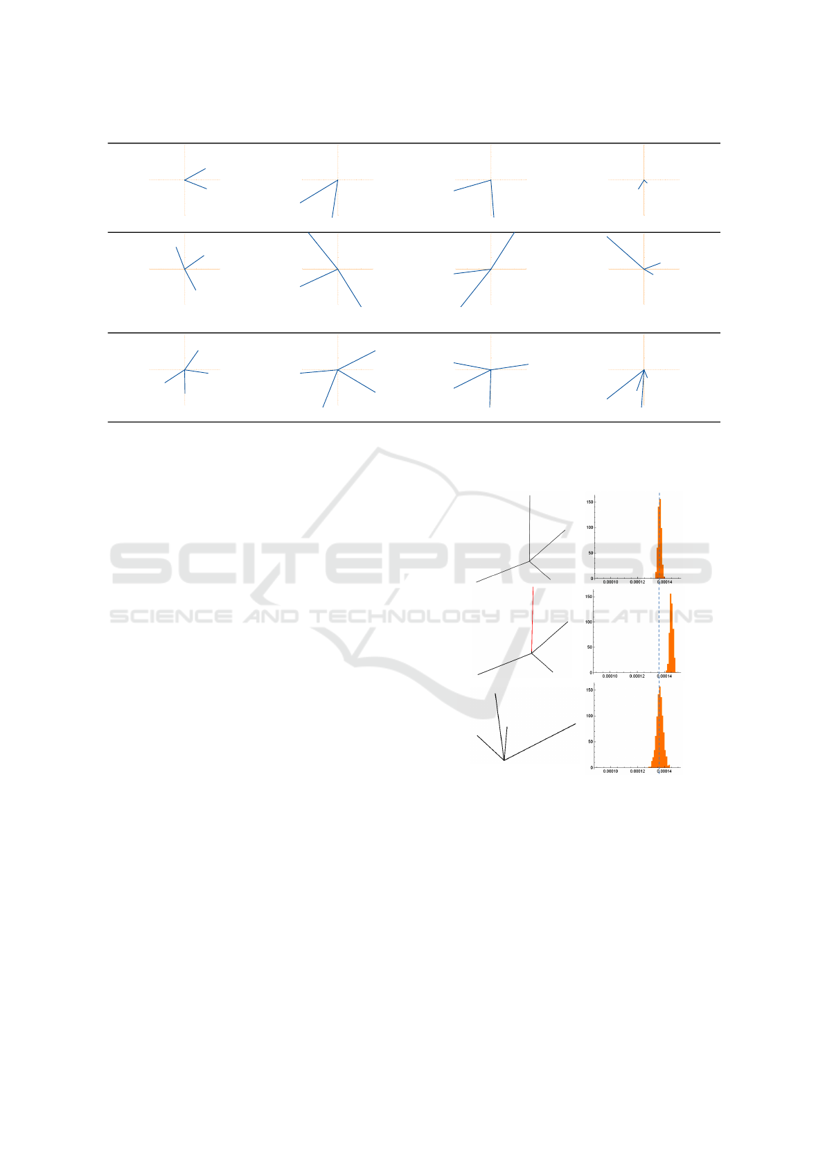
To demonstrate the distinctiveness of the given

projective invariant monomial, we built continuous

4-junctions and their projective-transformed counter-

parts (see Fig. 2). For each digital version of each

junction, we took its central and delimiter pixels and

produced 100,000 random continuous junctions by

sampling points in the pixels’ area. Then, we com-

puted the histogram of α numbers related to the set

of random samples and compared the histograms of

original and transformed junctions. Fig. 2 (top) il-

lustrates junctions used as reference and histograms

of invariant values produced using the random sam-

ples. Notice that there is a well-deﬁned peak of votes

close to the actual α number computed for the refer-

ence junction (the dashed line). The distribution of

random α samples produced for an unrelated junc-

tion generates a peak of votes in a different α value

(Fig. 2, middle), while the peak of votes generated

for the transformed version of the reference junction

preserves the signature of the distribution (Fig. 2, bot-

tom). Such behavior suggests that the histogram of

samples may be used to characterize well-deﬁned dis-

crete junctions related by projective transformations.

5 THE PROPOSED PROJECTIVE

INVARIANT DESCRIPTOR

The invariant numbers presented in Section 4 are de-

ﬁned for continuous junctions (J

) in bidimensional

The Recipe for Some Invariant Numbers and for a New Projective Invariant Feature Descriptor

185

Reference Similarity Transformation Afﬁne Transformation Projective Transformation

-1.5 -1.0 -0.5 0.5 1.0 1.5

-1.5

-1.0

-0.5

0.5

1.0

1.5

-1.5 -1.0 -0.5 0.5 1.0 1.5

-1.5

-1.0

-0.5

0.5

1.0

1.5

-1.5 -1.0 -0.5 0.5 1.0 1.5

-1.5

-1.0

-0.5

0.5

1.0

1.5

-1.5 -1.0 -0.5 0.5 1.0 1.5

-1.5

-1.0

-0.5

0.5

1.0

1.5

γ = 0.14821 γ = 0.14821 γ = 0.238821 γ = 0.143078

-1.5 -1.0 -0.5 0.5 1.0 1.5

-1.5

-1.0

-0.5

0.5

1.0

1.5

-1.5 -1.0 -0.5 0.5 1.0 1.5

-1.5

-1.0

-0.5

0.5

1.0

1.5

-1.5 -1.0 -0.5 0.5 1.0 1.5

-1.5

-1.0

-0.5

0.5

1.0

1.5

-1.5 -1.0 -0.5 0.5 1.0 1.5

-1.5

-1.0

-0.5

0.5

1.0

1.5

β =



0.15 0.16 0.00

0.13 0.13 0.00



β =



0.15 0.16 0.00

0.13 0.13 0.00



β =



0.15 0.16 0.00

0.13 0.13 0.00



β =



0.02 0.22 0.01

0.01 0.22 0.01



-1.5 -1.0 -0.5 0.5 1.0 1.5

-1.5

-1.0

-0.5

0.5

1.0

1.5

-1.5 -1.0 -0.5 0.5 1.0 1.5

-1.5

-1.0

-0.5

0.5

1.0

1.5

-1.5 -1.0 -0.5 0.5 1.0 1.5

-1.5

-1.0

-0.5

0.5

1.0

1.5

-1.5 -1.0 -0.5 0.5 1.0 1.5

-1.5

-1.0

-0.5

0.5

1.0

1.5

α = 0.496638 α = 0.496638 α = 0.496638 α = 0.496638

Figure 1: Each row presents one type of junction transformed by similarity, afﬁne, and projective transformations (columns).

The respective invariant value, γ, β, and α is at the bottom of each sample junction. Blue and red texts denote when the value

remains the same or changed after the transformation of the reference junctions.

intensity images (I ). For a given bidimensional inten-

sity digital image

I : Z

7→ R

, the discrete domain

I leads to the deﬁnition of digital junctions as:

ˆp | ˆp ∈

,∃ i ∈ {1,2,. .., n}

where n ∈ {2,3,4} is the degree of the junction, and

denotes the set of pixels ˆp = (u,v) ∈ Z

deﬁning

the i-th branch of the junction having the central pixel

ˆp

∩

as the only pixel shared by the branches,

for all i 6= j and i, j ∈ {1,2,. .., n}. By deﬁnition, the

branches

are digital straight line segments ranging

from the central pixel ˆp

to the delimiter pixel ˆp

The challenges for deﬁning a projective invariant

junction descriptor include: (i) detect well-deﬁned 4-

junctions in images (Section 5.1); (ii) compute de-

scriptors for the detected junctions (Section 5.2); and

(iii) deﬁne a matching procedure (Section 5.3).

5.1 Detecting Junctions in Digital

Images

It is quite difﬁcult to perform accurate detection of

well-deﬁned 4-junctions in digital images of natural

scenes using computationally cheap procedures. Our

proposed strategy to accomplish this task is to ﬁnd

image corners using the Minimum Eigenvalue Cor-

ner Detector (Shi and Tomasi, 1994) and, for each de-

tected corner, deﬁne a region of interest (ROI) from

which the analysis of the gradient leads to the identiﬁ-

cation of candidate branches leaving the corner. Can-

didate 4-junctions are produced from the combination

Figure 2: The distributions of α numbers (right) computed

for random junctions samples produced from a digital junc-

tions (left). The junction in the bottom was created by ap-

plying a homography to the junction in the top. The junction

in the middle is not related to the others by a homography.

of those branches. Thus, instead of retrieve one digital

junction for each detected corner, we use each corner

as the central vertex of a set of junctions representing

the image gradient around it. Section 5.2 shows how

the α numbers related to these candidate junctions are

combined to produce a descriptor for the ROI.

VISAPP 2020 - 15th International Conference on Computer Vision Theory and Applications

186

5.2 Computing the Feature Descriptors

Our feature descriptor is a histogram having m bins,

which count the (weighted) frequency of invariant

numbers computed for the set of digital junctions.

However, our experience shows that α numbers close

zero are more frequent (see Fig. 3, left). As a re-

sult, a histogram on the observations of α having a

small m might be unrepresentative (i.e., all resultant

histograms would look the same). We have overcome

this issue by performing a non-linear order-preserving

bijective mapping α 7→

α based on the theoretical cu-

mulative distribution of α. Fig. 3 (right) shows the

frequency distribution of

α numbers computed from

the α values assumed in Fig. 3 (left). Note that fre-

quencies are better distributed along with the

α axis.

Without loss of generality, let

α =

det(PP)

(PP)

≡



1 + µ

+ µ



(13)

be the invariant number deﬁned in (10) rewritten in

terms of 1 ≥ µ

≥ µ

≥ 0, where 1, µ

, and µ

are

the eigenvalues of the symmetric matrix PP after be-

ing divided by the eigenvalue with the largest mag-

nitude (recall that scaling PP does not affect α). Us-

ing (13), it is possible to conclude that α ∈ [0,1/27],

since max

,µ

α = 1/27. Also, (13) allows us to deﬁne the

theoretical cumulative distribution function of α as:

F (α) = 1 − 2

˙µ

(α)

(µ

− ˙µ

(µ

,α)) dµ

where functions ˙µ

and ˙µ

are obtained by solv-

ing (13) for µ

= µ

and µ

= 1, respectively.

For a given α number, we map it to

α using:

α = F (α), (14)

where

α ∈ [0, 1]. We use numerical integration to

evaluate F and its inverse, and keep a lookup list with

m entries to perform fast mapping between α and

α.

Each histogram assigned to a given corner pixel

ˆc is computed as follows: (i) each digital junction

is approximated by the continuous junction J

whose

vertices correspond to the center of the endpixels of

; (ii) the α value of each J

is computed using (10)

and mapped to

α using (14); (iii) the

α values con-

tribute to the ﬁnal histogram according to the weight

of their respective digital junctions, which is com-

puted as the product of the strength of the branches.

5.3 Matching Procedure

Given two sets of invariant histograms, namely

A and B, we use the k-Nearest Neighbors algo-

rithm (k -NN) (Friedman et al., 1977) to ﬁnd the best

0.001 0.002 0.003 0.004 0.005 0.006 0.007

α0

500

1000

1500

2000

Count

0.2 0.4 0.6 0.8 1.0



200

400

600

800

Count

Figure 3: Distribution of α numbers before (left) and af-

ter (right) applying the non-linear mapping α 7→

α. The fre-

quencies concentrate on the left side of the α domain. After

mapping, they distribute better in the [0,1] domain of

α.

match in A for each descriptor in B. In our experi-

ments, we have assumed k = 1 and the Earth Mover’s

Distance (EMD) (Rubner et al., 1998) to compare two

histograms. Alternatively, any other algorithms could

be used to match our feature histogram, as long as an

appropriate distance metric is adopted (e.g., Kullback-

Leibler Divergence and Chi-Squared Test).

6 CONCLUSIONS

In this paper, we presented how to compute symmet-

ric matrices from the geometry of junctions having

degree two or three, and how to use these matrices

with monomials invariant to, respectively, similarity

and afﬁne transformations. Using the cross-ratio, we

showed how to compute a projective invariant num-

ber for ideal junctions having degree four. Also, we

presented the derivation of a new projective invariant

number for 4-junctions, which is independent of the

cyclic order assumed for the branches of the junction

and to the normalization of the homogeneous coordi-

nate in projective space. Using the latter invariant,

we deﬁned a new procedure for detecting, describ-

ing, and matching local projective invariant junction-

based features in digital images.

Results show that our descriptor is promising

since it is capable of representing discriminative in-

formation. Unfortunately, the practical attempts to

implement the projective descriptor in natural images

failed due to several reasons, most of them related

to ﬁnding digital 4-junctions, which is an open re-

search topic, and that’s why we did not perform com-

parisons with state-of-the-art techniques. We are cur-

rently investigating ways to improve the detection of

junctions’ vertices in digital images. We hope that by

showing connections between the junction’s geome-

try and existing invariant monomials and by present-

ing new invariant numbers and a new descriptor, this

work may stimulate further researches.

The Recipe for Some Invariant Numbers and for a New Projective Invariant Feature Descriptor

187

ACKNOWLEDGEMENTS

This work was partially supported by CNPq-

Brazil (grant 311.037/2017-8) and FAPERJ (grant

E-26/202.718/2018) agencies. Raphael was spon-

sored by a CAPES fellowship.

REFERENCES

Alajlan, N., El Rube, I., Kamel, M. S., and Freeman, G.

(2007). Shape retrieval using triangle-area represen-

tation and dynamic space warping. Pattern Recogn.,

40(7):1911–1920.

Alajlan, N., Kamel, M. S., and Freeman, G. (2006). Multi-

object image retrieval based on shape and topology.

Image Commun., 21(10):904–918.

Aldana-Iuit, J., Mishkin, D., Chum, O., and Matas, J.

(2016). In the saddle: Chasing fast and repeatable

features. In ICPR, pages 675–680.

Balntas, V., Riba, E., Ponsa, D., and Mikolajczyk, K.

(2016). Learning local feature descriptors with triplets

and shallow convolutional neural networks. In BMVC.

Barrow, H. G. and Tenenbaum, J. M. (1981). Interpreting

line drawings as three-dimensional surfaces. Artif. In-

tell., 17(1-3):75–116.

Bay, H., Ess, A., Tuytelaars, T., and Van Gool, L. (2008).

Speeded-up robust features (SURF). Comput. Vis. Im-

age Underst., 110(3):346–359.

Biederman, I. (1985). Human image understanding: recent

research and a theory. Computer Vision, Graphics,

and Image Processing, 32:29–73.

Bosch, A., Zisserman, A., and Muñoz, X. (2008). Scene

classiﬁcation using a hybrid generative/discriminative

approach. IEEE Trans. Pattern Anal. Mach. Intell.,

30(4):712–727.

Calonder, M., Lepetit, V., Ozuysal, M., Trzcinski, T.,

Strecha, C., and Fua, P. (2012). BRIEF: Computing

a local binary descriptor very fast. IEEE Trans. Pat-

tern Anal. Mach. Intell., 34(7):1281–1298.

Cayley, A. (1858). A memoir on the theory of matrices.

Phil. Trans., 148:17–37.

Fan, X., Luo, Z., Zhang, J., Zhou, X., Jia, Q., and Luo, D.

(2014). Characteristic number: Theory and its appli-

cation to shape analysis. Axioms, 3:202–221.

Forsyth, D., Mundy, J. L., and Zisserman, A. (1991). In-

variant descriptors for 3D object recognition and pose.

IEEE Trans. Pattern Anal. Mach. Intell., pages 971–

991.

Friedman, J. H., Bentely, J., and Finkel, R. A. (1977). An

algorithm for ﬁnding best matches in logarithmic ex-

pected time. ACM Trans. Math. Softw., 3(3):209–226.

Gdalyahu, Y. and Weinshall, D. (1999). Flexible syntactic

matching of curves and its application to automatic

hierarchical classiﬁcation of silhouettes. IEEE Trans.

Pattern Anal. Mach. Intell., 21(12):1312–1328.

Hartley, R. I. and Zisserman, A. (2004). Multiple View Ge-

ometry in Computer Vision. Cambridge University

Press, 2nd edition.

Jia, Q., Fan, X., Liu, Y., Li, H., Luo, Z., and Guo, H.

(2016). Hierarchical projective invariant contexts for

shape recognition. Pattern Recognit., 52:358–374.

Ke, Y. and Sukthankar, R. (2004). PCA-SIFT: A more dis-

tinctive representation for local image descriptors. In

CVPR, pages 506–513.

Li, E., Mo, H., Xu, D., and Li, H. (2019). Image projective

invariants. IEEE Trans. Pattern Anal. Mach. Intell.,

41(5):1144–1157.

Lindeberg, T. (2012). Scale selection properties of gener-

alized scale-space interest point detectors. J. Math.

Imaging Vision, 46(2):177–210.

Lowe, D. G. (1999). Object recognition from local scale-

invariant features. In ICCV, pages 1150–1157.

Luo, Z., Luo, D., Fan, X., Zhou, X., and Jia, Q. (2013). A

shape descriptor based on new projective invariants.

In ICIP, pages 2862–2866.

Mishchuk, A., Mishkin, D., Radenovi

c, F., and Matas, J.

(2017). Working hard to know your neighbor’s mar-

gins: Local descriptor learning loss. In NIPS, pages

4829–4840.

Perwass, C. and Forstner, W. (2006). Uncertain Geome-

try with Circles, Spheres and Conics, pages 23–41.

Springer Netherlands.

Quan, L. (1995). Invariant of a pair of non-coplanar con-

ics in space: deﬁnition, geometric interpretation and

computation. In ICCV, pages 926–931.

Quan, L., Gros, P., and Mohr, R. (1991). Invariants of a pair

of conics revisited. In BMVC, pages 71–77.

Rosten, E. and Drummond, T. (2006). Machine learning for

high-speed corner detection. In ECCV, pages 430–

443.

Rosten, E., Porter, R., and Drummond, T. (2010). Faster and

better: a machine learning approach to corner detec-

tion. IEEE Trans. Pattern Anal. Mach. Intell., 32:105–

119.

Rubner, Y., Tomasi, C., and Guibas, L. J. (1998). A metric

for distributions with applications to image databases.

In ICCV, pages 59–66.

Semple, J. G. and Kneebone, G. T. (1952). Algebraic Pro-

jective Geometry. Oxford Science Publication.

Shi, J. and Tomasi, C. (1994). Good features to track. In

CVPR, pages 593–600.

Tian, Y., Fan, B., and Wu, F. a. (2017). L2-Net: deep learn-

ing of discriminative patch descriptor in Euclidean

space. In CVPR, pages 6128–6136.

Tian, Y., Yu, X., Fan, B., Wu, F., Heijnen, H., and Balntas,

V. (2019). SOSNet: second order similarity regular-

ization for local descriptor learning. In CVPR, pages

11016–11025.

Tuytelaars, T. and Mikolajczyk, K. (2008). Local invariant

feature detectors: A survey. Found. Trends. Comput.

Graph. Vis., 3(3):177–280.

Yu, G. and Morel, J. (2011). ASIFT: An algorithm for fully

afﬁne invariant comparison. IPOL, 1:11–38.

VISAPP 2020 - 15th International Conference on Computer Vision Theory and Applications

188