Radially Distorted Planar Motion Compatible Homographies

Marcus Valtonen

Ornhag

Centre for Mathematical Sciences, Lund University, Lund, Sweden

Keywords:

Planar Motion, Homography, Radial Distortion, Polynomial Solver, Trajectory Recovery, Visual Odometry.

Abstract:

Fast and accurate homography estimation is essential to many computer vision applications, including scene

degenerate cases and planarity detection. Such cases arise naturally in man-made environments, and failure

to handle them will result in poor positioning estimates. Most modern day consumer cameras are affected

by some level of radial distortion, which must be compensated for in order to get accurate estimates. This

often demands calibration procedures, with speciﬁc scene requirements, and off-line processing. In this paper

a novel polynomial solver for radially distorted planar motion compatible homographies is presented. The

proposed algorithm is fast and numerically stable, and is proven on both synthetic and real data to work well

inside a RANSAC loop.

1 INTRODUCTION

In many computer vision applications it is desired

to ﬁnd a homography between two images. With-

out imposing any prior knowledge of the model, or

intrinsic parameters, a general homography can be

estimated using a minimal of four point correspon-

dences (Hartley and Zisserman, 2004). If any of the

intrinsic parameters are known, or other model con-

straints are enforced, the number of needed point cor-

respondences decrease, however, encoding these ge-

ometric properties may result in non-linear systems

of polynomial equations. Solving such systems suf-

ﬁciently fast, with an acceptable numerical precision,

often involves methods from computational algebraic

geometry (Cox et al., 2005).

Planar motion models are a well-studied ﬁeld in

computer vision. While several authors have con-

sidered restricted models, requiring various calibra-

tion procedures (Ort

ın and Montiel, 2001; Chen and

Liu, 2006; Hajjdiab and Lagani

ere, 2004), the general

case, including the assumption of a constant—and

unknown—overhead tilt, was introduced in (Liang

and Pears, 2002). This model was also considered

by (Wadenb

ack and Heyden, 2013; Wadenb

ack and

Heyden, 2014; Zienkiewicz and Davison, 2015).

Many planar motion compatible navigation sys-

tems are based on estimating the homographies for

consecutive views. Instead of eight degrees of free-

dom, as in the general case, planar motion compatible

homographies only have ﬁve—two overhead tilt an-

gles (assumed to be constant), one rotational angle,

and two translational components. The standard pro-

cedure for estimating homographies is usually divided

in extracting and matching keypoints, followed by

estimating putative homographies in a robust frame-

work. Typically, this is done using RANSAC in or-

der to discard outliers introduced in the matching step.

The probability of selecting a set of points containing

only inliers depends on the amount of points selected,

and therefore it is advantageous to make this choice

minimal.

In this paper we consider the case of planar motion

with a constant overhead tilt and unknown radial dis-

tortion. Such a setup is common for Visual Odometry

(VO) in man-made environments, where the goal is to

estimate the position of a vehicle, on which the cam-

era is mounted. We propose a novel four point homo-

graphy solver, which is suitable for real-time applica-

tions and numerically stable. The solver is compared

to an existing solver and show an increase in perfor-

mance on both synthetic and real data. Furthermore,

we show how the solver can be incorporated in a VO

pipeline for indoor navigation.

2 RELATED WORK

Consider a pair of point correspondences x

x ↔

x, on

a common scene plane, related by a homography H

In homogeneous coordinates, let x

x = (x, y, w)

and

x = ( ˆx, ˆy, ˆw)

, then λ

x = H

x, for some scalar λ. Left-

280

Örnhag, M.

Radially Distorted Planar Motion Compatible Homographies.

DOI: 10.5220/0008893802800288

In Proceedings of the 9th International Conference on Pattern Recognition Applications and Methods (ICPRAM 2020), pages 280-288

ISBN: 978-989-758-397-1; ISSN: 2184-4313

multiplying this relation with the cross-product ma-

trix [

gives [

x = 0

0, or, equivalently,





0 − ˆwx

ˆyx

ˆwx

0 − ˆxx

− ˆyx

ˆxx













= 0

0, (1)

where h

is the k:th row of the homography ma-

trix H

H. This formulation conveniently eliminates the

scale parameter λ, while introducing two linearly in-

dependent equations, since the cross-product matrix

is of rank 2. These are known as the Direct Linear

Transform (DLT) equations. From this formulation,

using four point correspondences, the minimal prob-

lem reduces to ﬁnding the one-dimensional null space

of H

H. If the homography is constrained further, as

in the case of planar motion, this approach can still

be used; however, the null space is no longer one-

dimensional. The problem then translates into ﬁnd-

ing the corresponding null space basis coefﬁcients.

In (Wadenb

ack et al., 2016) the authors showed that

it was possible to construct a minimal solver for the

general planar motion homography by using this ap-

proach, in which a polynomial system of 11 quartic

equations in four variables are solved. Non-minimal

relaxations of the same problem was studied in (Val-

tonen

Ornhag, 2019), and tested in a VO framework

for planar motion.

There are two common approaches for modeling

radial distortion, the Brown–Conrady model (Brown,

1966), and the division model introduced in (Fitzgib-

bon, 2001). The latter has the beneﬁt of being suf-

ﬁciently good with fewer parameters than the for-

mer. We will exclusively use the division model

with a single distortion parameter λ, in which the

distorted (measured) image points are denoted x





, and related to the undistorted image

points x

, by the relation

= f (x

,λ) =





1 + λ(x

+ y

)





. (2)

where the distortion center is assumed to be at the

center of the image, which is also the origin of our se-

lected coordinate system. Since the distortion param-

eter only appears in the homogeneous coordinates, the

DLT equations (1) still hold true, with the adjustment

[ f (

,λ)]

H f (x

,λ) = 0

0, (3)

for two point correspondences x

↔

. A minimal

solver for the case of radially distorted homographies

were presented in (Kukelova et al., 2015), in which

the authors incorporated the radial distortion using

the modiﬁed DLT equations (3). The same approach,

but explicitly parameterizing the homography, have

been used in (Pritts et al., 2018a), where the authors

consider the case of conjugate translations. The case

of jointly estimating lens distortion and afﬁne recti-

ﬁcation from coplanar features, was studied in (Pritts

et al., 2018b). All the above methods reduce the prob-

lem to a polynomial system of equation for which the

action matrix method is used (Cox et al., 2005). This

typically involves ﬁnding a Gr

obner basis, and ex-

tracting template coefﬁcients in a ﬁnite ﬁeld, which

can be tedious manual work. Luckily, there are auto-

matic solvers, such as the ones presented in (Kukelova

et al., 2008a; Larsson and

Astr

om, 2016; Larsson

et al., 2017a; Larsson et al., 2017b; Larsson et al.,

2018b), from which the above mentioned radially dis-

torted homography solvers are derived.

An alternative to Gr

obner basis methods is to

view the problem as a Quadratic Eigenvalue Prob-

lem (QEP). This was done in (Fitzgibbon, 2001) and

the same approach has been used by (Kukelova et al.,

2008b; Kayumbi and Cavallaro, 2008).

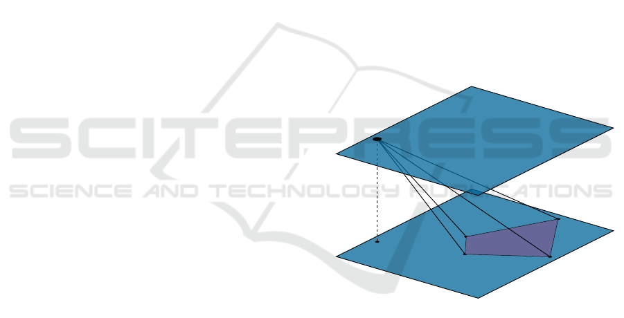
z = 1

z = 0

Figure 1: Illustration of the problem geometry. The ground

plane is assumed to be positioned at z = 1, and the camera

travels parallel in the plane z = 0. There are two unknown

overhead tilt angles ψ (x-axis) and θi (y-axis), which are

constant throughout the trajectory.

3 MODEL ASSUMPTIONS

We consider the original problem formulation

in (Wadenb

ack and Heyden, 2013), which assumes

that a camera directed towards the ﬂoor is mounted

on a vehicle. The scale of the global coordinate sys-

tem is ﬁxed by selecting the ground plane at z = 1, and

the camera is assumed to travel parallel to the ground,

in the plane z = 0, see Figure 1. Then, the camera

matrices for two consecutive poses A and B, are given

Radially Distorted Planar Motion Compatible Homographies

281

−20

−10

·10

−2

|λ − λ

est

Frequency (%)

−20

−10

·10

−2

H − H

est

Frequency (%)

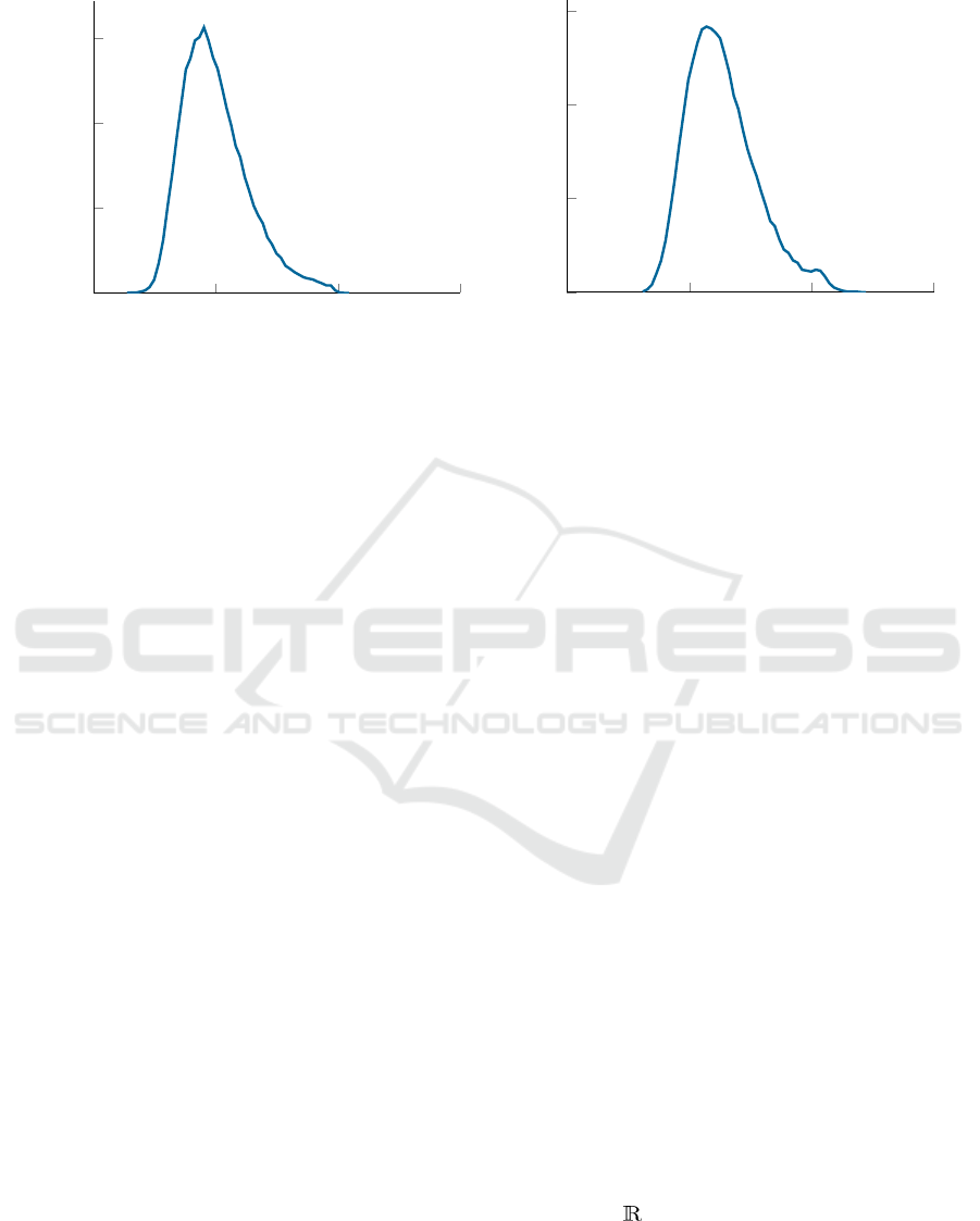
Figure 2: Error histogram the estimated distortion parameter λ (left) and the homography H

H for 100,000 random instances.

= R

ψθ

I | 0

0],

= R

ψθ

I | − t

t],

(4)

where R

ψθ

is a rotation θ about the y-axis followed by

a rotation of ψ about the x-axis. The vehicle may ro-

tate about the z-axis by an angle φ, modeled by R

and translate in the plane z = 0, thus leaving two

translation components t

and t

. The corresponding

homography is given by

H = λR

ψθ

, (5)

where T

= I

I − t

is a translation matrix, for the

translation t

t =





, relative the plane nor-

mal n

n =



0 0 1



In (Wadenb

ack et al., 2016) it was shown that a

planar motion compatible homography H

H must fulﬁll

11 quartic constraints. Later, it was shown that by

adding a sextic constraint, these conditions are both

necessary and sufﬁcient (Valtonen

Ornhag, 2019).

4 NON-MINIMAL RELAXATION

Note that there are six degrees of freedom in the

formulation—ﬁve in the planar motion compatible

homography and one from the distortion parameter—

hence using three points are required for the minimal

conﬁguration. This problem is surprisingly hard, and

we have not found any tractable solution, which yields

a solver sufﬁciently fast and stable for real-life scenar-

ios. Instead, we propose a non-minimal relaxation,

using four point correspondences. We argue that this

compromise is acceptable, as the minimal case for a

radially distorted general homography is 4.5 points

(thus requiring 5 points in practice).

We draw inspiration from the approach

in (Kukelova et al., 2015), however, we con-

sider using only four point correspondences. By

expanding the third row of (3), one obtains

(− ˆy

+ ˆx

+ (− ˆy

+ ˆx

(− ˆy

+ ˆx

= 0,

(6)

where w

= 1 + λ(x

+ y

) and ˆw

= 1 + λ( ˆx

+ ˆy

)

are both functions of the radial distortion parameter λ.

This is a homogeneous equation in eight monomials



λh



. (7)

With four point correspondences these can be stacked

= 0

0, (8)

where M

is a 4× 8 matrix, and v

is deﬁned as in (7).

Hence, in general, the null space of M

is four dimen-

sional, and we may parameterize v

∑

i=1

, (9)

where γ

are the new unknowns. To ﬁx the scale we let

= 1. Since the elements of v

are not independent,

one needs to enforce two constraints, namely,

= λv

and v

= λv

. (10)

Next, consider the second row of (3), which can be

written

= 0

0, (11)

where M

∈

4×16

, with the null space vector v

con-

sisting of 7 variables, and 16 monomials: h

, h

, λh

and λ

, λγ

, γ

for i = 1, 2,3 and λ

, λ, 1.

Since there are four equations with the same monomi-

als we can eliminate the three ﬁrst variables, h

, h

ICPRAM 2020 - 9th International Conference on Pattern Recognition Applications and Methods

282

−3

−2.5

−2

−1.5

−1

−0.5

−7

−5

−3

−1

|λ − λ

est

−3

−2.5

−2

−1.5

−1

−0.5

−3

−2

−1

kH − H

est

Proposed (4-pt)

Fitzgibbon (5-pt)

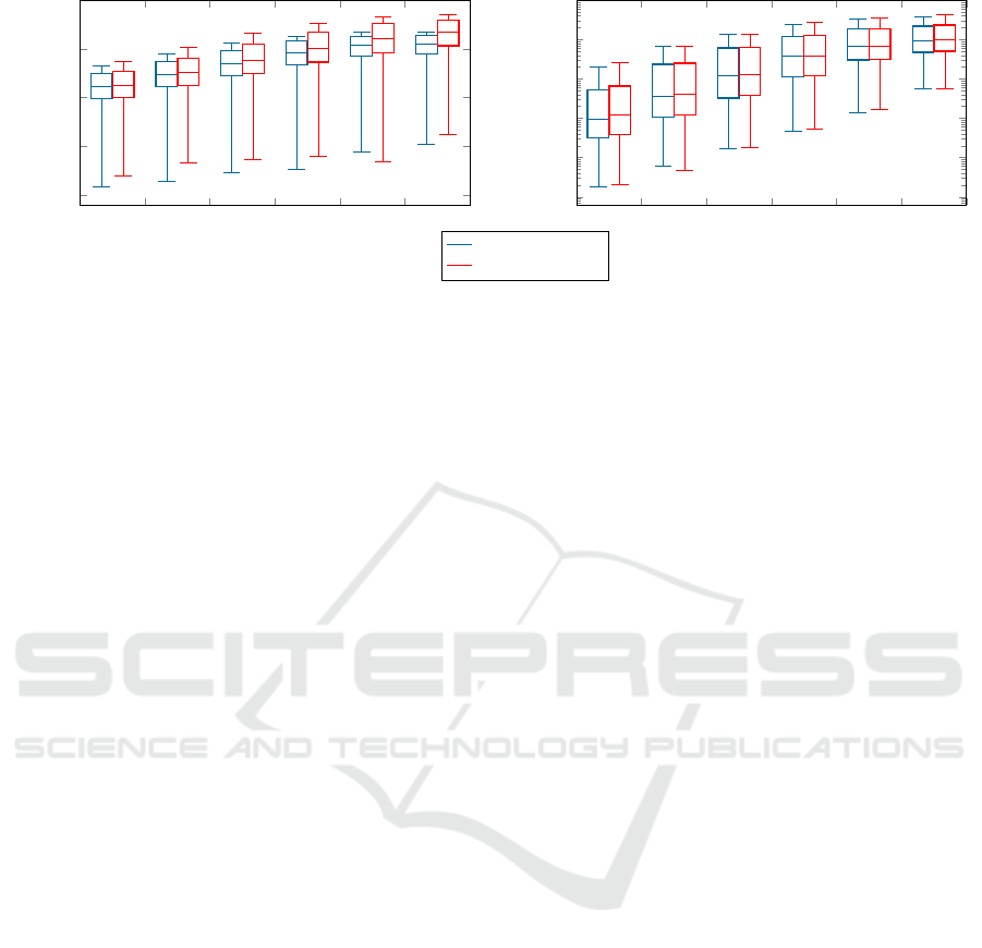
Figure 3: Distribution of estimation error in the distortion parameter λ, and the the homography H

H (measured in the Frobenius

norm) for different noise levels σ. The proposed solver is compared to the ﬁve point solver (Fitzgibbon, 2001).

and h

, using Gauss-Jordan elimination. Performing

the elimination we obtain







λh

λγ

λ 1

1 • • • ··· • • •

1 • • • · ·· • • •

1 • • • ·· · • • •







(12)

where we notice that the columns of the right 4 × 12

submatrix are not independent. In order to generate

a correct solver, it is important to generate integer in-

stances satisfying these dependencies.

From the eliminated system

= 0

0 we get the

four equations.

+ f

(γ

,γ

,λ) = 0,

+ f

(γ

,γ

,λ) = 0,

λh

+ f

(γ

,γ

,λ) = 0,

+ f

(γ

,γ

,λ) = 0,

(13)

where f

(γ

,γ

,λ) are polynomials in the variables

, γ

, λ. Exploiting the relations between the last

two equations of (13), an additional constraint is ob-

tained

λ f

(γ

,γ

,λ) = f

(γ

,γ

,λ) . (14)

The eliminated variables h

, h

and h

are polyno-

mials of degree three, thus making (14) of degree four.

Together with (10) we have three equations in four

unknowns. Since we are able to express all elements

of the homography H

H as a function of four variables,

we can enforce one of the 11 quartic constraints orig-

inally found in (Wadenb

ack et al., 2016). Evaluating

these constraints using H

H it turns out that ten of the

constraints are of degree 12 and one of degree 10 due

to cancellation of higher order terms. We choose the

smallest one to build the polynomial solver.

Using the automatic generator (Larsson and

Astr

om, 2016) we ﬁnd that there are 18 solutions to

the problem in general, and by sampling a basis based

on the heuristic presented in (Larsson et al., 2018a) an

elimination template of size 177 × 195 could be cre-

ated.

5 EXPERIMENTS

5.1 Synthetic Data

The performance of the new polynomial solver is an-

alyzed in terms of numerical stability and noise sen-

sitivity. This is done by generating planar motion

compatible homographies and distortion parameters.

Scene points are generated and corresponding points

are mapped using the previously generated homogra-

phies, followed by radially distorting the points using

the division model.

The polynomial solver was generated according to

Section 4 in C++, and the mean run-time is 0.73 ms

(measured over 10,000 instances on a standard desk-

top computer).

5.1.1 Numerical Stability

We generate noise-free problem instances as de-

scribed in the previous section, with physically rea-

sonable parameters. As in (Kukelova et al., 2015)

the distortion parameter λ was chosen in the inter-

val [−0.7,0], which covers a wide range of distor-

tions. The error histogram for 100,000 random in-

stances are shown in Figure 2. The homographies

were normalized such that h

= 1. The majority

of estimated distortion parameters λ are in the error

range of 10

−10

which is acceptable for most applica-

tions; however, there are still a signiﬁcant parameter

estimates of an error in the order of 10

−2

or more,

which is not negligible. This is likely to stem from

Radially Distorted Planar Motion Compatible Homographies

283

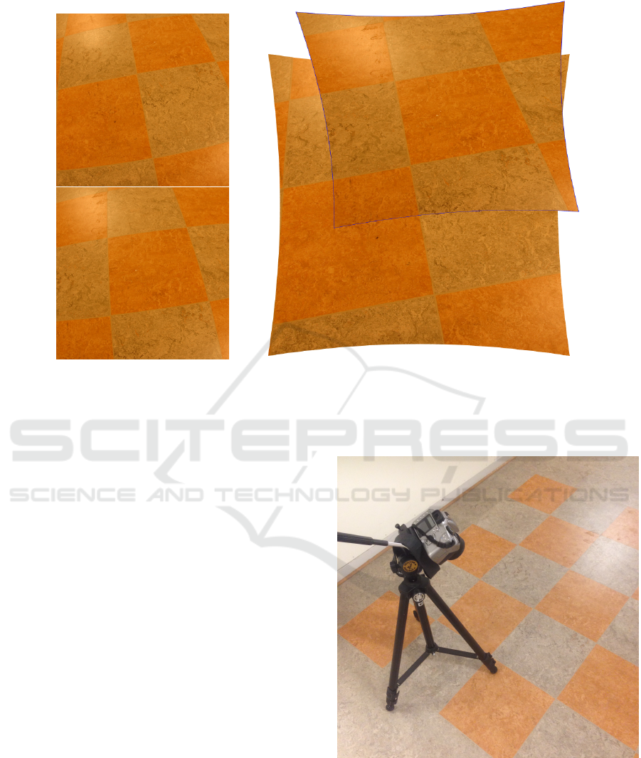
Input

Output

Figure 4: Two radially distorted images (left) and the rectiﬁed and stitched panorama. The distortion parameter and homo-

graphy was obtained using the proposed solver in a RANSAC framework. Blue border added for visualization.

the ten degree polynomial, which increases the resid-

ual error notably. Nevertheless, we show that, care-

fully incorporated in a RANSAC framework, this is

still a viable option to existing methods.

5.1.2 Noise Sensitivity

To analyze how well the solver copes with noise, the

radially distorted image coordinates were corrupted

by Gaussian noise with standard deviation σ, vary-

ing from mild to severe noise (in percent). The test

was conducted 10,000 times per noise level, see Fig-

ure 3. As a comparison we use the ﬁve point method

proposed in (Fitzgibbon, 2001). For all noise levels

the mean error for the distortion parameter λ and the

homography H

H, obtained using the proposed solver,

are lower compared to the ﬁve point method.

5.2 Real Images

5.2.1 Image Stitching

Stitching of images is a classic problem in computer

vision. In this section, we show that the proposed

method yields a visually acceptable output from real

data.

The images were taken using a digital camera with

a ﬁsh-eye lens mounted on a tripod, see Figure 5.

The overhead tilt was kept ﬁxed and the entire tripod

moved along the ﬂoor, thus creating a planar motion

compatible homography between the images.

Figure 5: Setup used in the panorama stitching experiment.

We use a standard approach for estimating the

homography. First we detect and extract SURF key-

points, followed by matching them using the near-

est neighbor algorithm. Outliers are removed in a

RANSAC framework. No non-linear reﬁnement of

the obtained homography was performed. The ﬁnal

ICPRAM 2020 - 9th International Conference on Pattern Recognition Applications and Methods

284

−5

·10

−7

100

150

∗

est

Frequency

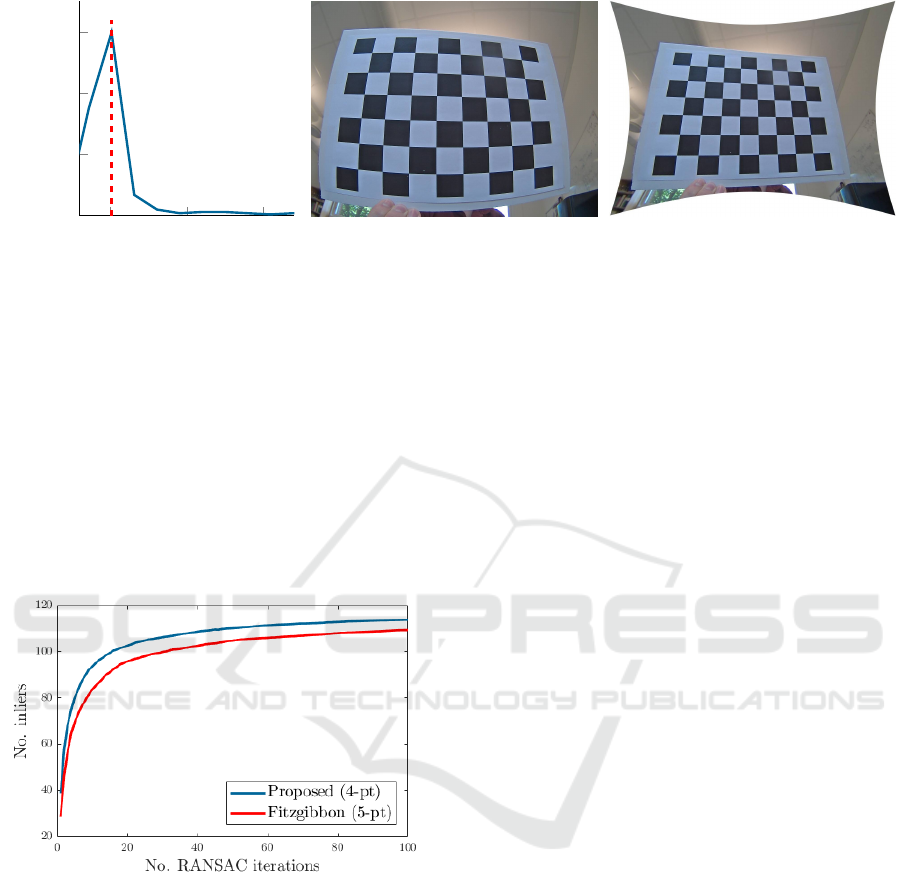
Figure 6: (Left) Histogram of estimated distortion parameters for the proposed method evaluating during the parallel parking

sequence. The selected parameter λ

∗

is marked with a dashed line. (Middle) Undistorted image of a calibration chart, not part

of the sequence. (Right) Rectiﬁed image using the estimated parameter λ

∗

panorama can be seen in Figure 4. Note that the

lines appear straight in the ﬁnal output, indicating that

the radial distortion parameter has been correctly es-

timated. In Figure 7 we compare the number of in-

liers vs. number of RANSAC iterations for the same

image pair, using the proposed method and the ﬁve

point solver in (Fitzgibbon, 2001). In the experiment

we mean-value the number of inliers over 500 prob-

lem instances, and the proposed method consistently

has a higher number of inliers.

Figure 7: Number of inliers vs. number of RANSAC itera-

tions for the images in Figure 4. The data has been mean-

valued over 500 test instances.

5.2.2 Application to Visual Odometry

In this ﬁnal section we show that the proposed solver

can be incorporated in a VO pipeline to achieve bet-

ter performance to the compared method. The clas-

sic pipeline consists of constructing an initial solution

for the camera poses, intrinsic parameters and scene

points, and then reﬁne these using Bundle Adjustment

(BA). In general, if a better initial solution can be ob-

tained, fewer iterations of BA are needed for the same

performance. As the latter step often amounts in a

large optimization step, it is certainly advantageous

to decrease the number of necessary iterations.

In this experiment we use the data from the mo-

bile robot experiment in (Wadenb

ack et al., 2017).

The robot is equipped with omnidirectional wheels

(Fraunhofer IPA rob@work) and has a camera (with

visible radial distortion) mounted downwards, such

that the ﬂoor is predominantly in the ﬁeld of view.

Reference images of a calibration pattern (checker-

board) are taken as a sanity check of the estimated

distortion parameter. Furthermore, a reference sys-

tem with an absolute accuracy of 100 µm is set up to

track the platform, from which the ground truth data

is obtained.

The robot is programmed with three sequences,

described below:

Line. Forward motion in a straight line with a con-

stant orientation (320 images),

Turn. Forward motion while rotating, resulting in a

slight turn (344 images),

Parallel Parking. Forward motion followed by a

sharp turn, while keeping constant rotation (325

images).

As in the stitching experiment in the previous sec-

tion we compare the proposed method to the one

in (Fitzgibbon, 2001). For each pair of consecu-

tive images a homography and a radial distortion pa-

rameter are estimated using both methods. Then the

method in (Wadenb

ack and Heyden, 2014) is used

to recover the full set of motion parameters. From

these the trajectory of the robot is extracted and com-

pared to the ground truth, see Figure 8. Both meth-

ods perform well, with a slight preference for the pro-

posed method. This result is consistent with the ﬁnd-

ings in (Valtonen

Ornhag, 2019); namely, that pre-

optimization on an early stage in the VO pipeline,

does not lead to a signiﬁcant performance boost. This

is, in large, due to the constraint that the constant

overhead tilt throughout the entire trajectory cannot

be enforced on a single homography alone, but rather

Radially Distorted Planar Motion Compatible Homographies

285

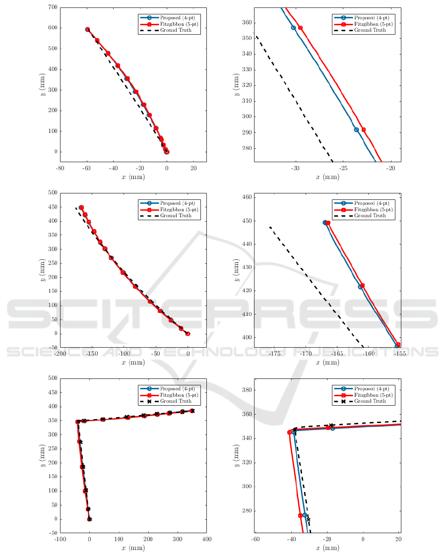
Figure 8: Estimated trajectories for line, turn and parallel parking of the VO experiment in Section 5.2.2. Images to the left

show the entire trajectory, and the ones to the right are zoomed in on a region of interest.

requires a sequence of homographies. Nevertheless,

there is still the same performance gain in terms

of the number of RANSAC iterations needed to ac-

quire a given inlier ratio, as was demonstrated in Sec-

tion 5.2.1.

The presented experiment does not enforce the

ICPRAM 2020 - 9th International Conference on Pattern Recognition Applications and Methods

286

same radial distortion parameter throughout the tra-

jectory of the robot, as it estimates a new parameter

along with each homography. In order to enforce the

same radial distortion compensation, we may use his-

togram voting of the estimated distortion parameters.

In Figure 6 we have done so for the estimated para-

meters acquired during the parallel parking test se-

quence. The most likely parameter λ

∗

is then used to

rectify a previously unseen image of the calibration

scene. While the rectiﬁed image is not perfect, it may

serve as a good initial solution for further non-linear

reﬁnement.

6 CONCLUSIONS

One cannot ignore radial distortion when estimat-

ing trajectories in a Visual Odometry framework. In

this paper we have considered radially distorted ho-

mographies compatible with the general planar mo-

tion model. We have proposed a novel algorithm

for estimating the homographies and showed on both

real and synthetic data that it increases the perfor-

mance compared to a general homography estima-

tion method with radial distortion. Furthermore, we

show, by incorporating the proposed algorithm in a

VO pipeline, that it yields satisfactory results in terms

of estimating the radial distortion parameter.

ACKNOWLEDGMENTS

The author gratefully acknowledges M

arten

Wadenb

ack and Martin Karlsson for providing

the data for the planar motion compatible sequences,

and Magnus Oskarsson for fruitful discussions

regarding the basis selection heuristic which made

the proposed solver faster. This work has been

funded by the Swedish Research Council through

grant no. 2015-05639 ‘Visual SLAM based on Planar

Homographies’.

REFERENCES

Brown, D. C. (1966). Decentering distortion of lenses. Pho-

togrammetric Engineering, 32:444–462.

Chen, T. and Liu, Y.-H. (2006). A robust approach for struc-

ture from planar motion by stereo image sequences.

Machine Vision and Applications (MVA), 17(3):197–

209.

Cox, D. A., Little, J., and O’Shea, D. (2005). Using Al-

gebraic Geometry. Graduate Texts in Mathematics.

Springer New York.

Fitzgibbon, A. W. (2001). Simultaneous linear estimation of

multiple view geometry and lens distortion. In Con-

ference on Computer Vision and Pattern Recognition

(CVPR).

Hajjdiab, H. and Lagani

ere, R. (2004). Vision-based multi-

robot simultaneous localization and mapping. In

Canadian Conference on Computer and Robot Vision

(CRV), pages 155–162, London, ON, Canada.

Hartley, R. I. and Zisserman, A. (2004). Multiple View Ge-

ometry in Computer Vision. Cambridge University

Press, Cambridge, England, UK, second edition.

Kayumbi, G. and Cavallaro, A. (2008). Multiview trajec-

tory mapping using homography with lens distortion

correction. EURASIP Journal on Image and Video

Processing, page 145715.

Kukelova, Z., Bujnak, M., and Pajdla, T. (2008a). Auto-

matic generator of minimal problem solvers. Euro-

pean Conference on Computer Vision (ECCV), pages

302–315.

Kukelova, Z., Bujnak, M., and Pajdla, T. (2008b). Polyno-

mial eigenvalue solutions to the 5-pt and 6-pt relative

pose problems. In British Machine Vision Conference

(BMVC).

Kukelova, Z., Heller, J., Bujnak, M., and Pajdla, T. (2015).

Radial distortion homography. In Conference on Com-

puter Vision and Pattern Recognition (CVPR), pages

639–647.

Larsson, V. and

Astr

om, K. (2016). Uncovering symme-

tries in polynomial systems. European Conference on

Computer Vision (ECCV), pages 252–267.

Larsson, V.,

Astr

om, K., and Oskarsson, M. (2017a). Ef-

ﬁcient solvers for minimal problems by syzygy-based

reduction. Computer Vision and Pattern Recognition

(CVPR), pages 2383–2392.

Larsson, V.,

Astr

om, K., and Oskarsson, M. (2017b). Poly-

nomial solvers for saturated ideals. International

Conference on Computer Vision (ICCV), pages 2307–

2316.

Larsson, V., Kukelova, Z., and Zheng, Y. (2018a). Camera

pose estimation with unknown principal point. Com-

puter Vision and Pattern Recognition (CVPR), pages

2984–2992.

Larsson, V., Oskarsson, M.,

Astr

om, K., Wallis, A.,

Kukelova, Z., and Pajdla, T. (2018b). Beyond gr

obner

bases: Basis selection for minimal solvers. Computer

Vision and Pattern Recognition (CVPR), pages 3945–

3954.

Liang, B. and Pears, N. (2002). Visual navigation using

planar homographies. In International Conference

on Robotics and Automation (ICRA), pages 205–210,

Washington, DC, USA.

Ort

ın, D. and Montiel, J. M. M. (2001). Indoor robot motion

based on monocular images. Robotica, 19(3):331–

342.

Pritts, J., Kukelova, Z., Larsson, V., and Chum, O. (2018a).

Radially-distorted conjugate translations. In Confer-

ence on Computer Vision and Pattern Recognition

(CVPR).

Pritts, J., Kukelova, Z., Larsson, V., and Chum, O. (2018b).

Radially Distorted Planar Motion Compatible Homographies

287

Rectiﬁcation from radially-distorted scales. In Asian

Conference of Computer Vision (ACCV), pages 36–52.

Valtonen

Ornhag, M. (2019). Fast non-minimal solvers for

planar motion compatible homographies. In Inter-

national Conference on Pattern Recognition Applica-

tions and Methods (ICPRAM), pages 40–51, Prague,

Czech Republic.

Wadenb

ack, M. and Heyden, A. (2013). Planar motion and

hand-eye calibration using inter-image homographies

from a planar scene. International Conference on

Computer Vision Theory and Applications (VISAPP),

pages 164–168.

Wadenb

ack, M. and Heyden, A. (2014). Ego-motion recov-

ery and robust tilt estimation for planar motion using

several homographies. International Conference on

Computer Vision Theory and Applications (VISAPP),

pages 635–639.

Wadenb

ack, M., Karlsson, M., Heyden, A., Robertsson, A.,

and Johansson, R. (2017). Visual odometry from two

point correspondences and initial automatic tilt cali-

bration. In International Joint Conference on Com-

puter Vision, Imaging and Computer Graphics Theory

and Applications (VISIGRAPP 2017), pages 340–346.

Wadenb

ack, M.,

Astr

om, K., and Heyden, A. (2016). Re-

covering planar motion from homographies obtained

using a 2.5-point solver for a polynomial system. In-

ternational Conference on Image Processing (ICIP),

pages 2966–2970.

Zienkiewicz, J. and Davison, A. J. (2015). Extrinsics auto-

calibration for dense planar visual odometry. Journal

of Field Robotics (JFR), 32(5):803–825.

ICPRAM 2020 - 9th International Conference on Pattern Recognition Applications and Methods

288