
The Effect of Maxblur-pooling in Neural Networks on Shift-invariance
Issue in Various Biological Signal Classification Tasks
Xianyin Hu, Shangyin Zou, Yuki Ban and Shin’ichi Warisawa
Development of Human and Engineered Environmental Studies, The Graduate School of Frontier Sciences,
The University of Tokyo, Kashiwa, Chiba, Japan
Keywords:
Temporal Shift-invariance, Maxblur-pooling, Neural Network, Bio-signal Processing, Atrial Fibrillation (AF)
Detection, Emotion Recognition.
Abstract:
Modern neural networks are widely employed in bio-signal processing due to their effectiveness. However, re-
cent research showed that neural networks for image recognition is not shift-invariant as it was assumed, while
it is an important property in bio-signal processing. Fortunately, a simple methodology was proposed referred
to as Maxblur-pooling to improve the shift-invariance of neural networks for image recognition. However, the
corresponding issue in the domain of bio-signal processing remains untouched. To verify the shift-invariance
of neural networks when applied to bio-signal processing, we performed two experiments across different
tasks and types of bio-signals. One is Atrial Fibrillation (AF) detection from R-R interval and the other is
emotion recognition from multi-channel EEG. We were able to show that the lack of shift-invariance also hap-
pens in temporal bio-signal classification. In the AF detection task, we succeed to validate the effectiveness of
Maxblur-pooling, which demonstrating improvements in both accuracy (2%-13%) and consistency (8%-15%)
compared to the baseline. While for the emotion recognition task, we did not observe any improvements using
Maxblur-pooling. Our research provided empirical knowledge for developing real-time diagnose systems that
is stable to temporal shifts.
1 INTRODUCTION
Deep learning approaches have achieved great suc-
cess in the field of image recognition and natural lan-
guage processing. In recent years, deep neural net-
works are also widely employed in biosignal process-
ing served as feature extractors and pattern classifiers.
For example, the most commonly investigated bio-
signal is electrocardiogram (ECG). Work by Acharya
et al. (Acharya et al., 2017) used an 11-layer deep
CNN to automatically detect arrhythmias. Another
popular field of bio-signal classification using neural
networks is Electroencephalogram (EEG). Tripathi et
al. applied deep neural networks and convolutional
neural networks to emotion recognition and gained
rather high accuracy (Tripathi et al., 2017).
In most of the automatic diagnosis systems mod-
eled as bio-signal classification task, there are usually
two steps, the first step is feature extraction and the
second step is pattern classification. In the first step,
temporal shift-invariance, also referred to as time in-
variance or translation invariance (Mitra and Kaiser,
1993), is required. Temporal shift-invariance sim-
ply means that if you shift the input signal along
the time axis by an arbitrary amount, as long as the
ground truth does not change, all the features ex-
tracted should also stay the same. The ideal extracted
features should be only related to the final target while
remaining irrelevant to time. That is, the contempo-
raneous features extracted from a given series of the
input raw signals should not depend on when the in-
put occurs.
Someone may get confused with the state-
ment:temporal shift-invariance is expected in biosig-
nal processing. They may consider the change in-
stead of the invariance should be expected since there
exists so many analysis performed on moving win-
dows to track the temporal evolution. In fact, mod-
els that do biosignal classification tasks are exactly
time-invariant systems. It can be easily understand
by comparing between time-variant system and time-
invariant system. In a time-variant system, for the
same input that happens at differnt time, the out-
put is different. In a time-invariant system, for the
same input that happens at differnt time, the output
is the same. The temporal evolution to be tracked
is not the evolution of the time itself, but the evolu-
tion of the parameters and behaviors in the input sig-
nals along the time. According to the definition of
time-invariant system (Oppenheim, 1997), if a classi-
fier depends only indirectly on the time-domain (via
the input function, for example), then that is a sys-
Hu, X., Zou, S., Ban, Y. and Warisawa, S.
The Effect of Maxblur-pooling in Neural Networks on Shift-invariance Issue in Various Biological Signal Classification Tasks.
DOI: 10.5220/0008879900490059
In Proceedings of the 13th International Joint Conference on Biomedical Engineering Systems and Technologies (BIOSTEC 2020) - Volume 4: BIOSIGNALS, pages 49-59
ISBN: 978-989-758-398-8; ISSN: 2184-4305
Copyright
c
2022 by SCITEPRESS – Science and Technology Publications, Lda. All rights reserved
49

Figure 1: The temporal shift-invariance is lacked in modern neural networks for AF detection task and Maxblur-
pooling technique improved shift-invariance. The horizontal axis is the shift offset applied to the input RRI segment and
the vertical axis is the probability of making the correct estimation. We observed a drastic change of the confidence in the
output of the baseline model using Max-pooling while the output of the model using Maxblur-pooling is more stable. This
figure generated from the outputs of 151-th RRI segment to 251-th RRI segment in the recording of No.07162. (Referring to
the expression S(x
i
, k) in Figure.3, here i = 151 and k = 1, 2, 3, . . . , 99).
tem that would be considered time-invariant. In our
cases, biosignal classifiers depend only indirectly on
the time-domain via the biosignals (time-dependent
function). Thus, the biosignal classifiers satisfied the
definition and should be modeled as time-invariance
systems.
Temporal shift-invariance is always addressed in
the traditional analysis method in biosignal process-
ing. For example, the discrete wavelet transform
(DWT) is a commonly used time-frequency anal-
ysis and signal-coding tool to extract suitable fea-
tures from raw biosignals (Addison et al., 2009),
but it is also well-known for its drawbacks of lack-
ing temporal shift-invariance. To solve the prob-
lem, a set of methods was proposed to overcome the
problem to maintain temporal shift-invariance, such
as the stationary wavelet transform (SWT) (Addison
et al., 2009), adaptive wavelet transform (Xiong et al.,
2000), etc.
Maintaining a high temporal shift-invariance is es-
pecially important and a challenging issue in devel-
oping real-time disease diagnosis systems. Real-time
analysis of patient data during medical procedures can
provide vital diagnostic feedback that significantly
improves chances of success. The term ”real-time”
means the system should response immediately to the
input. In other words, the real-time system is required
to output a stream with a sampling rate that is same
with or near to the sampling rate of its input signal. If
the system has low temporal shift-invariance, the out-
put will suffer drastic change even when the input is
shifted by a very small offset, which is not desirable.
Although the temporal shift-invariance has been
addressed in traditional analysis methods of biosig-
nals, researchers utilized modern neural network tech-
nology have neglected this important property. The
reason is that these researchers take it for granted
that the neural network approach is temporal shift-
invariant and does not verify that.
In fact, in the first place, the basic structures that
make up modern neural networks are designed un-
der the motivation of maintaining shift-invariance.
Proceeding researches believed that neural networks
can acquire shift-invariance from both the architec-
ture and the parameter.
For the way of acquiring from the architecture,
layers with shared weights and layers of downsam-
pling are proposed. For example, in convolutional
neural networks (CNN), the weights of the filters in
convolution layers are shared across all patches of the
image - so the weights learned can be invariant to po-
sition. And max-pooling layer, by taking the max
value of the pixel in the patch, approximate transla-
tion invariance can be gained since subsequent layers
of the CNN don’t care about the specific position in
the patch that the max value was in. Similarly, in re-
current neural networks (RNN), weights are shared
across time to gain temporal shift-invariance.
For the way of acquiring from parameter, a com-
monly used approach is to do data augmentation by
adding shifted data into the training set, then expect
the weights of the neural networks to learn shift-
invariance from the large amount of data.
It has been recently proved in the task of im-
age recognition that the neural network is not shift-
invariant as we expected (Azulay and Weiss, 2019).
However, in the field of biosignal processing, the cor-
responding issue remained untouched. Therefore, it
is necessary to verify whether the neural networks ap-
plied in bio-signal processing also lack temporal shift-
invariance.
A novel methodology named Maxblur-pooling
BIOSIGNALS 2020 - 13th International Conference on Bio-inspired Systems and Signal Processing
50

Figure 2: Testbeds selection criteria. A situation when the
duration of onset symptom is less than segment length and
we will not select the task to be our testbed. We denoted
S(x
i
, s) as given the input segment x
i
a temporal shift s. Al-
though the shifted segment S(x
i
, 1) contains the symptom,
the shfited segment S(x
i
, s) doesn’t.
was proposed by Zhang to overcome the drawback
of lacking shift-invariance in modern neural networks
(Zhang, 2019). This method has been validated in
the task of image recognition and image generation
across several challenging datasets such as ImageNet.
Zhang held that shift-invariance is lost because of the
down-sampling in the pooling layer. However, shift-
invariance can be simply fixed if features are extracted
densely. This motivated them to break the Max-
pooling layer in modern neural networks into two op-
erations: (1) evaluating the max operator densely and
(2) naive subsampling. They proposed to add low-
pass (Gaussian) filters between them as a means of
anti-aliasing. This viewpoint enables low-pass fil-
tering to augment, rather than replace Max-pooling
layers. As a result, they proved the anti-aliasing
and Max-pooling can be combined in a novel way
and shifts in the input leave the output relatively
unaffected (shift-invariance). Although this method
gained success in the task of image recognition, there
is no guarantee that this method could generalize well
to the neural networks that process biosignals for the
following two reasons. Firstly, the Gaussian low-
pass filter of Maxblur-pooling is widely used in im-
age processing served as a smoothing filter, while
in the bio-signal processing, most of the researches
use Savitzky-Golay filter (Savitzky and Golay, 1964)
to smooth the bio-signals. The Savitzky-Golay fil-
ter is widely used for its main advantage to preserve
features of the signal such as maxima, minima, and
width, which are usually flattened by the Gaussian
filter. Secondly, concerning the frequency domain
analysis, the low-pass filter of Maxblur-pooling has a
side-effect that cut off some high-frequency compo-
nents. In image processing, high-frequency com-
ponents are usually conceived noise or are not nec-
essary for the recognition and should be filtered.
While in biosignals processing, although it’s case by
case, a large range of frequency components should
be taken into account. We concerned the Maxblur-
pooling employing the low-pass Gaussian filter may
lose important features of signals such as maxima and
high-frequency components for bio-signal processing
tasks, so we can’t say it certain that it will also im-
prove when applied to bio-signals.
Thus, the effectiveness of Maxblur-pooling and its
generalizability to biosignal processing is under dis-
cussion and needed validation.
In this work, we performed experiments on two
datasets using different biosignal, one is atrial fibril-
lation (AF) detection from R-R interval and the other
is effective estimation from EEG. The contributions
can be summarized as follows:
• We showed the problem that neural networks
lack shift-invariance also happens when tackling
with biosignals. As demonstrated in Fig. 1, out-
puts of the baseline neural network using max-
pooling suffer drastic changes according to tem-
poral shifts.
• We showed that Maxblur-pooling improved accu-
racy (2%-13%), as well as consistency (8%-15%)
in the task of AF detection, compared to the base-
line using max-pooling.
• We did not observe improvements between the
Maxblur-pooling and the baseline in the task of
affective estimation, indicating that this method
performed poorly to process the EEG signal. The
reason was discussed that the blurring behavior
of Maxblur-pooling lost too much information on
the high-frequency components which is neces-
sary for the effective estimation to estimate human
emotion.
• Our work provided empirical knowledge for de-
veloping and designing neural networks for real-
time diagnose systems that is stable and robust to
temporal shifts.
2 TESTBEDS & EVALUATION
In this section, we described the two testbeds selected
to perform the validation and the selection criteria.
Then we described the metrics to evaluate the effec-
tiveness of the Maxblur-pooling method.
The Effect of Maxblur-pooling in Neural Networks on Shift-invariance Issue in Various Biological Signal Classification Tasks
51

2.1 Testbeds Selection Criteria
Our criteria to select proper testbeds was as follows:
1) The task is to do biological signal classification.
2) The duration of the true onset symptoms must be
longer than the segment length of the input signal in
the dataset.
In Fig. 2 we demonstrated an example of how a
testbed does not satisfy our criteria. When the du-
ration of symptom onsets is less than the segment
length, it will happen that a shifted segment doesn’t
contain symptoms. So in such a task, we will never
know the ground truth of each shifted segment.
The tasks in which different output labels were
annotated between sessions satisfy the criteria. For
example, in emotion recognition, participants were
asked to watch videos that evoke various emotions.
The time of watching a video served as a session. In
this case, the duration of a session, also known as the
duration of onset symptoms, is always longer than the
segment length. For the tasks that can have differ-
ent labels inside one session, investigation of the task
itself is needed to determine whether it satisfies the
criteria. Here we take the sleep apnea detection as
an example that does not reach the criteria. In the
task of sleep apnea detection (Penzel et al., 2000),
the ground truth indicating the presence or absence of
apnea was annotated by human experts by every one
minute. Apnea is defined to happen when complete
pauses in breathing appear lasting at least 10 seconds
during sleep. However, the duration of onset symp-
tom (10 seconds) is much shorter than the segment
length which is one minute. So there is no guarantee
that the shifted ECG segment also contains the onset
symptom that makes it an apneic segment. Following
the above criteria, we selected two databases that can
be used for the verification of shift-invariance.
2.2 Testbeds
Atrial Fibrillation (AF) Detection. We used MIT-
BIH atrial fibrillation database (Moody, 1983) for the
task of atrial fibrillation (AF) detection. This database
includes 25 long-term ECG recordings of human sub-
jects with normal heart rhythm and atrial fibrillation.
The R peaks were annotated manually by human ex-
perts, so we can calculate R-R intervals from the an-
notated files directly without pre-processing. We used
100 R-R interval segments as input. Since the dura-
tion of atrial fibrillation usually lasts for hours or even
days, and the segment length is about less than two
minutes for 100 R-R intervals, the test-bed satisfies
the selection criteria.
Emotion Recognition. We adopted the public
SEED IV Emotion Dataset (Zheng et al., 2018) for
the task of emotion recognition. The SEED IV
dataset contains 62 channels of EEG and eye move-
ment data of four different emotions—happy, sad,
fear, and neutral. In this work, we used the EEG part
of the dataset. The EEG data is of 200Hz sampling
rate, obtained from a total of 15 subjects during ex-
perimental sessions conducted in 3 separate days. For
each emotion stimulation, the subjects were asked to
watch a two-minute video. Therefore EEG data of
a label is about two minutes as the length of videos.
Each span of EEG data was cut into 1-second seg-
ments as the input. As also mentioned in the above
subsection, the duration of emotion equals the dura-
tion of the session which is two minutes, longer than
the segment length of one second, so the test-bed also
satisfied the selecting criteria.
The two tasks selected uses different types of bio-
signal, so we can verify if the lack of shift-invariance
is a universal problem across bio-signal types and if
the Maxblur-pooling method generalizes well to var-
ious tasks. In each task, we tested five different blur
sizes ranged from 3 to 7 with the baseline using the
Max-pooling layer. In the first experiment on AF de-
tection, we also tested three different pooling factors,
denoted as p and p ∈ 1, 2, 3, p was also conceived to
be the number of pooling layers in the neural network.
Therefore, we tested three p-layer CNNs to find out
how the effect of Maxblur-pooling was influenced by
the pooling factor p.
2.3 Evaluation Metrics
The classification accuracy on the overall dataset (in-
cluding overlapped and non-overlapped segments) in-
tegrated the evaluation of how well the model per-
formed to make a correct estimation as well as how
much stable the model is. But the overall accuracy
failed to make a trade-off between the two aspects.
Zhang (Zhang, 2019) stated that the Maxblur-pooling
could improve the shift-invariance of a neural network
but may sacrifice accuracy. As a fact, he surprisingly
found that both accuracy and shift-invariance are im-
proved on the task of image classification and image
generation. For the purpose of the validation, we also
have to evaluate the two aspects separately. We de-
fined the accuracy and consistency as follows to eval-
uate the preciseness and shift-invariance of a model.
The accuracy is calculated based on the test dataset in
which all the segments are not overlapped with each
other. The consistency is defined based on shifted seg-
ments with an overlap less than L −1 between two ad-
jacent segments that have the same label (L equals to
the segment length).
BIOSIGNALS 2020 - 13th International Conference on Bio-inspired Systems and Signal Processing
52
The average value of both metrics are calculated
with 5-fold cross-validation. Higher accuracy indi-
cates a more accurate diagnose and higher consis-
tency indicates more shift-invariance.
Accuracy. Classification accuracy is defined
as the proportion of correct predictions to the
total number of predictions, denoting the pre-
dictions as a vector p = (p
1
, p
2
, p
3
, ..., p
n
)
T
=
( f (x
1
), f (x
2
), f (x
3
), ..., f (x
n
))
T
and the ground truth
as y = (y
1
, y
2
, y
3
, ..., y
n
)
T
. Accuracy can be defined
using the following equations:
α
i
=
(
1, if p
i
= y
i
0, otherwise
(1)
Accuracy =
1
n
n
∑
i=1
α
i
(2)
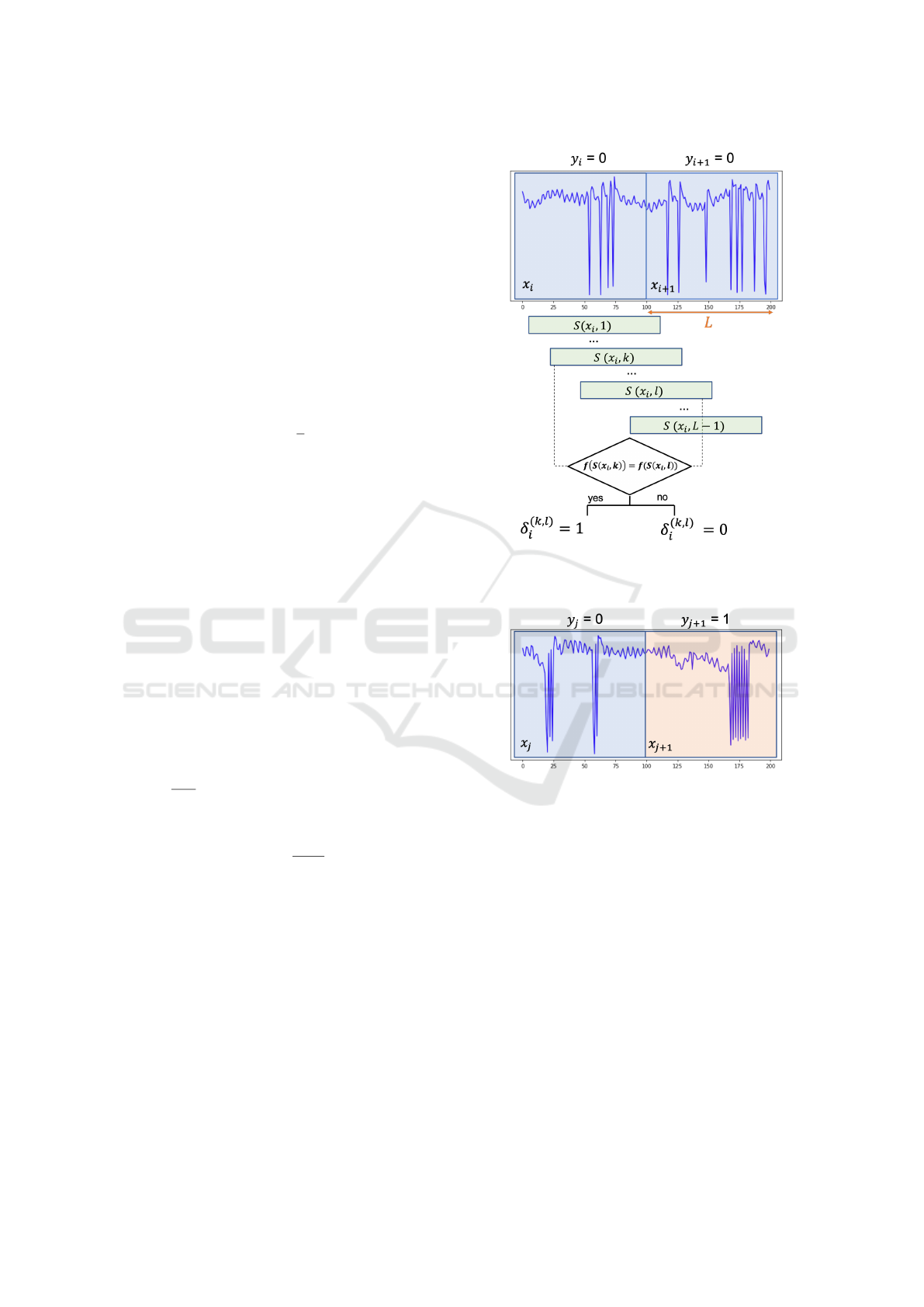
Consistency. The consistency checks how often the
network outputs the same label given the same input
bio-signal segment with two different temporal shifts.
For a piece of input segment, we denoted the segment
length as L, then there will be L − 1 shifts applied to-
tally. As demonstrated in Fig. 3(a), only the segments
that have the same label with its consecutively adja-
cent segment next in time will be used to calculate
consistency. For those segments that did not have the
same label with the next adjacent segment, shifts will
not be applied (Fig. 3(b)). We denoted S as the tempo-
ral shift function, and S(x, k) means temporally shift
the input x by an offset equals to k. The consistency
can be defined as follows:
δ
(k,l)
i
=
(
1, if f (S(x
i
, k)) = f (S((x
i
, l))
0, otherwise
(3)
δ
i
=
(
1
C
2
L−1
∑
k,l∈{1,...,L−1},k<l
δ
(k,l)
i
, y
i
= y
i+1
0, y
i
6= y
i+1
(4)
Consistency =
1
n − 1
n−1
∑
i=1
δ
i
(5)
3 VALIDATION ON ATRIAL
FIBRILLATION (AF)
DETECTION
3.1 Tested models
For the model structure, we adopted the basic convo-
lutional neural network (CNN) as is shown in Fig. 4.
The unit block of the CNN consisted of a convolution
layer, a batch normalization layer, a ReLU activation
(a) For the segment that had the same label with
its next adjacent segment, shifts will be applied and
consistency is calculated.
(b) For the segment that didn’t have the same label
with its next adjacent segment, shifts will not be ap-
plied.
Figure 3: Calculation of the consistency.
layer, and a pooling layer. The unit block will repeat
for p times, which equals to the pooling factor, and we
tested six variations of the pooling layers including
one baseline and Maxblur-pooling with five blur sizes
for comparison.
The input of the model is a 100 R-R intervals
sequence. Thanks to the contributors of the dataset
(Moody, 1983), we can calculate the R-R intervals
from the manually annotated heart rhythm without
pre-processing. The output of the model is a binary
value (0 or 1) indicating the presence or absence of
atrial fibrillation. We tested five different blur sizes
of Maxblur-pooling ranged from 3 to 7 together with
the baseline using Max-pooling. We also tested three
The Effect of Maxblur-pooling in Neural Networks on Shift-invariance Issue in Various Biological Signal Classification Tasks
53
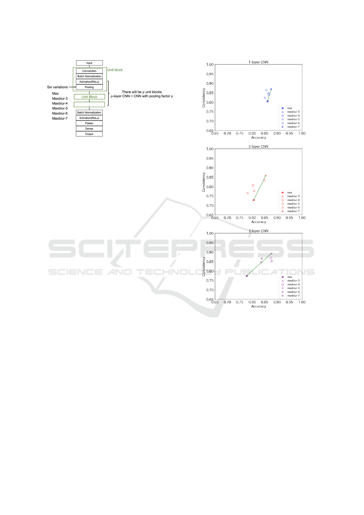
Figure 4: The structure of Convolution Neural Network
(CNN).
different pooling factors to find out how the effect of
Maxblur-pooling was influenced by the pooling fac-
tor.
3.2 Results and Discussion
We were able to reveal that the lack of temporal shift-
invariance also exists in modern neural networks in
the task of AF detection. As the example showed in
Fig. 1, we observed that outputs of the baseline model
using Max-pooling suffered from drastic changes as
the input shifted. By using the Maxblur-pooling, this
vibration of output had been significantly reduced.
The comparison results of CNN structures across
pooling factors were summarized in Table.1. To
demonstrate it more intuitively as shown in Fig. 5, the
upper right of the figure indicates better performance
on both metrics. We observed that all the models
using Maxblur-pooling with different blur sizes im-
proved consistency with various degrees compared to
the baseline of Max-pooling, but improvement in ac-
curacy was only observed with the blur size of 7 con-
sidering all the pooling factors.
For CNN with one layer, Maxblur-pooling with
blur size equaling to 7 obtained best results, which
improved accuracy by 1.72% and consistency by
7.94% compared to Max-pooling.
For CNN with two layers, Maxblur-pooling with
blur size equaling to 7 obtained best results, improv-
ing accuracy by 6.02% and consistency by 17.92%
compared to Max-pooling.
For CNN with three layers, Maxblur-pooling with
blur size equaling to 5 obtained best results, improv-
ing accuracy by 12.79% and consistency by 15.36%
compared to Max-pooling.
In the task of AF detection, we have observed that
Maxblur-pooling did improve accuracy and consis-
tency compared to Max-pooling. Although the best
performing filter varied by the pooling factor p, we
did not find there is a relationship between them. Em-
Figure 5: Performance of models for AF detection. In
each figure, the upper right indicates better performance on
both metrics. Points are plotted with different shapes cor-
responding to the variants of the networks using Maxblur-
pooling. The number of edges equals to the blur size (trian-
gle means Maxblur-pooling with blur size of 3). Specially,
star mark represents Maxblur-pooling with blur size of 7
and the alphabet M represents the baseline of Max-pooling.
pirically, we recommend using the blur size of 7 be-
cause it both improved accuracy and consistency in
all the three CNNs with different pooling factor.
Next, we discussed the relationship between the
improvement of Maxblur-pooling and how many
times the Maxblur-pooling was applied. As showed
in Fig. 6, when the pooling factor increased, improve-
ments in accuracy and consistency also increased.
Specifically, improvements of consistency in three-
layer CNN was significantly greater than that in one
BIOSIGNALS 2020 - 13th International Conference on Bio-inspired Systems and Signal Processing
54
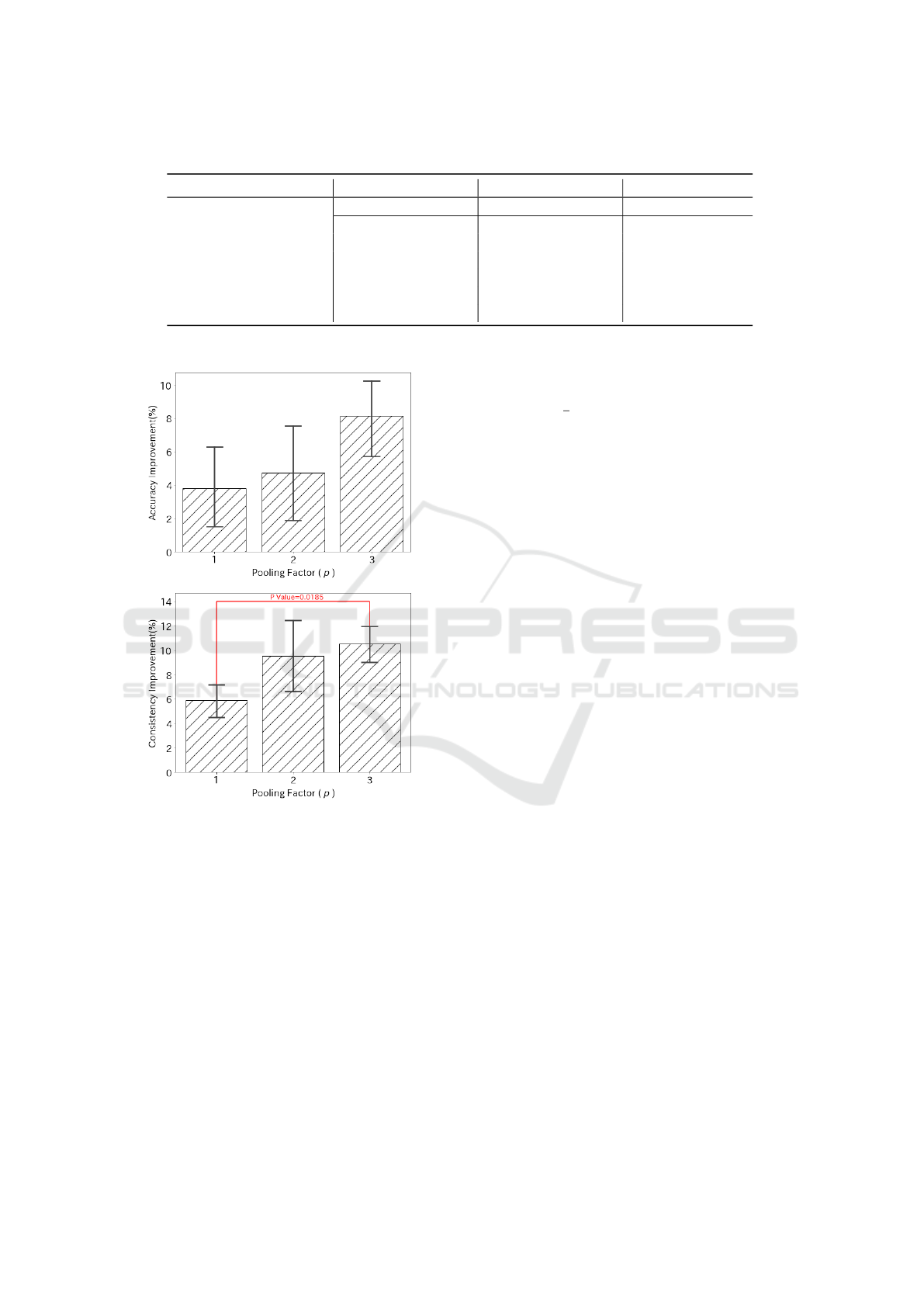
Table 1: Comparison between CNNs using different pooling layers for AF detection (accuracy and consistency are in %).
Task Pooling Layer 1-layer CNN 2-layer CNN 3-layer CNN
AF
Detection
accuracy consistency accuracy consistency accuracy consistey
Max 86.11 80.44 80.54 72.76 77.70 77.32
Maxblur-3 86.54 84.91 80.75 77.80 87.78 85.39
Maxblur-4 86.66 84.05 80.29 80.66 87.43 86.88
Maxblur-5 85.05 82.41 84.88 83.32 87.64 89.20
Maxblur-6 85.61 86.42 78.14 76.47 83.60 84.65
Maxblur-7 87.59 86.83 85.39 85.80 83.83 86.60
Figure 6: Improvements of Maxblur-pooling with differ-
ent pooling factors compared to the baseline. We com-
pared how much improvement was made by using Maxblur-
pooling from the baseline of Max-pooling between different
pooling factors. Tukey’s multiple comparison test was em-
ployed to check the significant difference (P value<0.05).
layer CNN, but a significant difference in improve-
ments of accuracy was not observed. Although the
number of pooling layers needed parameter-tuning
and is depended on the task and data. If shift-
invariance is especially desired, we suggest employ-
ing Maxblur-pooling in a deeper network with more
pooling layers.
4 EMOTION RECOGNITION ON
SEED IV EEG DATASET
4.1 Data Description
In the previous section, we discovered and discussed
that the problem of shift-variance exists in AF de-
tection 1-dimensional RRI data, and tested whether
the Maxblur-pooling layer will solve the problem by
replacing the traditional Max-pooling layer. We be-
lieved that the shift-variance problem should also ex-
ist in the recognition of 2-dimensional physiological
signals. Among many kinds of physiological signals,
we found Electroencephalography (EEG) signals are
one suitable type of 2-dimensional signal. This is be-
cause EEG signals are usually measured by multiple
channels; hence, there are the time dimension and the
channel dimension in EEG data. EEG signals also
have different characteristics than RRI data, for exam-
ple, EEG signals contain a wide frequency range from
1 Hz to at least 100 Hz. Previous studies on neural sci-
ence have discovered that different frequency ranges
of EEG show respective properties of brain activities
(Henry, 2006). Therefore, recognition tasks on EEG
require the model to capture information of a wide
range of frequencies.
Furthermore, the application of CNN in various
kinds of recognition from EEG signals has been a
widely investigated topic so that it will be meaningful
to verify the effectiveness of the Maxblur-pooling
layers. The deep learning models of CNN have been
applied to the detection of seizure from single EEG
signals (Acharya et al., 2018), emotion recognition
(Zheng and Lu, 2015; Mei and Xu, 2017) and
limb motion recognition (Zhang et al., 2018) from
multi-channel EEG, combined with feature extraction
methods or other deep learning model architecture
like Recurrent Neural Network (RNN) and long short-
term memory (LSTM) units. In Zhang’s research, the
Maxblur-pooling layers were originally proposed to
The Effect of Maxblur-pooling in Neural Networks on Shift-invariance Issue in Various Biological Signal Classification Tasks
55
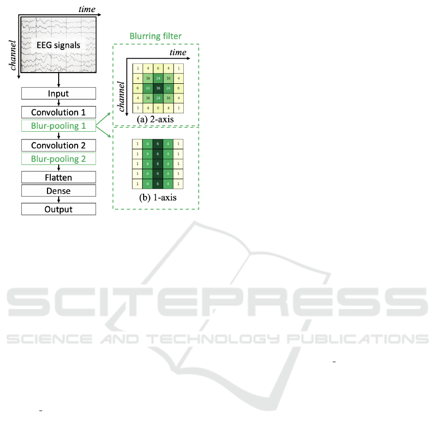
Figure 7: The architecture of the CNN model used for the
emotion recognition task. Two types of blur filters are also
illustrated. The horizontal axis represents the time series,
and the vertical represents channels. Here blur filters of size
5 are taken as examples. (a) is the 2-axis blur filter that has a
blurring effect on both temporal and channel axes, while (b)
is of 1 axis that only has a blurring effect on the temporal
axis.
solve the shift-variance problem of 2D images,
and the 2D blur filters were proved to be effective
against shift-variance of image recognition (Zhang,
2019). Therefore we anticipate that the Maxblur-
pooling layers in 2-dimensional CNN will also
improve the shift-invariance of the CNN models on
2-dimensional EEG data.
To verify this hypothesis, we adopted the pub-
lic SEED IV Emotion Dataset (Zheng et al., 2018)
for the task of discrete emotion recognition using the
CNN model.
4.2 Validation Procedure
Overall, we performed 5-fold cross-validation on
each participant, which means that the recognition
is participant-dependent. In the validation process
on EEG data, we used 1-second segments of EEG
raw data as the input to the CNN networks, which
was proved feasible by previous research (Yanagi-
moto and Sugimoto, 2016). Hence the input shape
of the network is (62, 200), where 62 is the number
of channels, and 200 is the total time frames of 1-
second segments. The reason that we did not use
any frequency-domain feature extraction method as
in most previous researches (Zheng et al., 2018) is
that we needed to keep the input data in the time do-
main in order to verify the temporal shifting effect of
Maxblur-pooling layers.
As for the model architecture, we adopted a CNN
model structure of 2 convolution layers, which was a
simple modified version based on previous researches
of emotion recognition using CNN from EEG (Mei
and Xu, 2017; Moon et al., 2018). The general ar-
chitecture is illustrated in Fig. 7, where the numbers
of filters of the two convolutional layers are 16 and
32, and the kernel size is (3, 3).The baseline model
structure is the same with normal Max-pooling layers
replacing the Maxblur-pooling layers.
Unlike image classification tasks, where the two
axes of a 2D image represent the same meaning, the
time axis and channel axis of EEG data include dif-
ferent information. We intend to find out whether
Maxblur-pooling layers will make improvements by
blurring along both time and channel axis, or only
along the time axis. Therefore we tested Maxblur-
pooling layers with two kinds of blur filters, as are
shown in Fig. 7 as filter (a) and (b). One has a blurring
effect on both time and channel axes, and the other
only blurs along the time axis, which is similar to 1D
blur filter. blur filter sizes of 3, 4, 5, 6, and 7, respec-
tively of the two types of blur filters were tested.
4.3 Results and Discussion
The validation procedure was still in process, and the
following results are based on data of 5 participants
among all 15 in the SEED IV dataset. The results of
mean accuracy and consistency are listed in Table.2.
For the comparison between two types of 2D blur fil-
ters, it was clear that 2-axis blurring outperformed 1-
axis blurring. The average accuracy and consistency
of 2-axis blurring of size from 3 to 7 were higher by
2.14% and 3.22% respectively than 1-axis blurring.
This shows that the blur filter on the channel axis im-
proved the recognition performance.
However, the best performance was gained by the
baseline model utilized Max-pooling layers, reached
an accuracy of 79.98% and consistency of 89.73%,
outperformed all the models with Maxblur-pooling
layers. On the contrary to our hypothesis, the appli-
cation of Maxblur-pooling in this task caused recog-
nition accuracy to drop about 6.28%, and consis-
tency dropped about 2.53% on average. These results
showed that the Maxblur-pooling layers performed
badly when processing EEG signals compared to
RRI, both accuracy-wise and consistency-wise. One
possible reason for this outcome we speculate is that
the filters in the Maxblur-pooling layers may have ex-
cluded some information contained in EEG signals
BIOSIGNALS 2020 - 13th International Conference on Bio-inspired Systems and Signal Processing
56
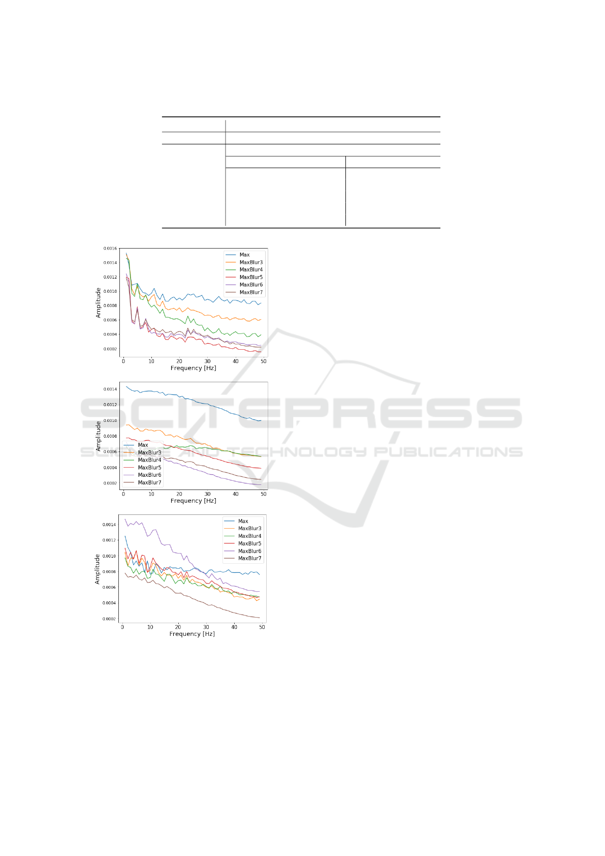
Table 2: Mean accuracy(%) and consistency(%) of two blur filters of the task of emotion recognition using EEG.
Pooling Layer
Max accuracy 79.98 consistency 89.73
2-axis blurring 1-axis blurring
accuracy consistency accuracy consistency
Maxblur-3 76.33 88.61 75.86 85.19
Maxblur-4 76.15 88.59 73.09 85.94
Maxblur-5 74.94 88.31 72.31 84.31
Maxblur-6 74.58 88.66 71.04 86.78
Maxblur-7 74.05 89.69 68.67 85.92
Figure 8: The FFT distribution of pooling layers’ output
feature. Three typical patterns are chosen.
that is important to emotions. This is because that,
as mentioned earlier, EEG signals cover a wide range
of frequencies, especially the gamma band (30-100
Hz) of which is crucial to emotion recognition, ac-
cording to previous research (Li and Lu, 2009). How-
ever, since the blur filters also served as low-pass fil-
ters, the reason for the low accuracy was considered
to be the fact that the Maxblur-pooling layers filtered
out the relatively high frequency components which
contained important information for emotion estimat-
ing, while Max-pooling layers maintained those in-
formation. Therefore applying Maxblur-pooling lay-
ers caused the accuracy to drop compared to Max-
pooling.
To verify the theory, we pulled out the output
matrices of the first pooling layer in the CNN net-
works from individual test samples, and conducted
FFT along the temporal axis to compare the frequency
distribution between normal Max-pooling layers and
Maxblur-pooling layers. Although the FFT distribu-
tion of the Maxblur-pooling features cannot fully rep-
resent the actual frequencies of EEG signals, we can
interpret the amplitude values as the amount of energy
and information. The outcomes of some typical pat-
terns are illustrated in Fig. 8. We noticed that among
the most of FFT distribution of test samples, the am-
plitude values of Max-pooling are the highest in the
30-50 Hz frequency range, while values of Maxblur-
pooling of larger sizes tend to be lower. This gives
us the indication that the Maxblur-pooling layers fil-
tered out more information contained in high frequen-
cies of EEG signals compared to Max-pooling layers.
As a result, the accuracy with Maxblur-pooling layers
dropped, and in the meantime, the consistency was
not improved.
5 GENERAL DISCUSSION
In the validation on AF detection task, we discussed
that the improvements of consistency in CNN with
more layers were significantly more than that in CNN
with fewer layers, but a significant difference in im-
provements of accuracy was not observed, suggest-
ing that deeper neural networks could be employed to
gain consistency.
The Effect of Maxblur-pooling in Neural Networks on Shift-invariance Issue in Various Biological Signal Classification Tasks
57

Table 3: Compare between CNNs using different pooling layers for AF detection with data augmentation (accuracy and
consistency are in %).
Task Pooling Layer 1-layer CNN 2-layer CNN 3-layer CNN
AF
Detection
accuracy consistency accuracy consistency accuracy consistey
Max 90.89 98.34 94.15 97.53 91.53 97.20
Maxblur-3 91.91 97.40 92.49 95.33 94.37 95.00
Maxblur-4 92.42 97.01 93.62 93.91 94.28 95.94
Maxblur-5 89.15 95.57 94.69 95.13 94.42 95.66
Maxblur-6 91.74 97.25 93.07 96.84 94.57 95.60
Maxblur-7 90.28 97.39 94.03 96.84 92.28 96.49
Figure 9: Results for AF detection using data augmentation.
We did not observe improvements.
In the validation on emotion recognition task,
Maxblur-pooling lost its advantage when applied to
EEG signals. We discussed the reason was to be
that the Maxblur-pooling layers filtered out the impor-
tant high-frequency components while normal Max-
pooling layers didn’t. Therefore applying Maxblur-
pooling layers caused the accuracy and consistency to
drop, indicating that this method is not suitable for
such tasks.
Before the method of Maxblur-pooling was pro-
posed, researchers usually use data augmentation to
gain shift-invariance. We compared the Maxblur-
pooling and baselines in the task of AF detection
with data augmentation to verify if Maxblur-pooling
can make improvements as well when the data was
augmented. As the result shown in Fig. 9, Using
Maxblur-pooling made no improvements in accuracy
and consistency from the baseline when applied with
data augmentation (Refer to Table.3 for details). We
considered the reason was that there left little room to
be improved within the task of AF detection. The per-
formance of the baseline model using Max-pooling
with data augmentation already reached an accuracy
of 94% and consistency of 98%. In other tasks that
could not gain high accuracy with data augmentation,
it’s worth trying Maxblur-pooling. Maxblur-pooling
could also exert its effect when data augmentation is
not possible in some online learning systems.
6 CONCLUSION
The objective of this work is to verify if the problem
of lacking shift-invariance also happens in neural net-
works that applied to bio-signals processing, and to
validate the effect of Maxblur-pooling methodology
in this field.
We succeeded to validate the lacking of shift-
invariance that also happens in modern neural net-
works applied in bio-signal processing. Besides, we
verified that the Maxblur-pooling method improved
accuracy and consistency in the task of AF detection
using RRI signal, but failed in the task of emotion
recognition using the EEG signal. In the tasks that are
BIOSIGNALS 2020 - 13th International Conference on Bio-inspired Systems and Signal Processing
58

similar to AF detection with RRI sequence as the in-
put signal, the results obtained indicate that Maxblur-
pooling, with a blur size of 7, should be used instead
of max-pooling. Moreover, if shift-invariance is espe-
cially desired, deeper networks with more Maxblur-
pooling is better. On the other hand, in the tasks
where high-frequency components are important, we
recommend to use the normal max-pooling layer. Fu-
ture work is to customize the Maxblur-pooling in a
way that is friendly to process bio-signals such as us-
ing the Avitzky-Golay filter instead of the Gaussian
filter.
REFERENCES
Acharya, U. R., Fujita, H., Lih, O. S., Hagiwara, Y., Tan,
J. H., and Adam, M. (2017). Automated detection
of arrhythmias using different intervals of tachycar-
dia ecg segments with convolutional neural network.
Information sciences, 405:81–90.
Acharya, U. R., Oh, S. L., Hagiwara, Y., Tan, J. H., and
Adeli, H. (2018). Deep convolutional neural network
for the automated detection and diagnosis of seizure
using eeg signals. Computers in biology and medicine,
100:270–278.
Addison, P. S., Walker, J., and Guido, R. C. (2009). Time–
frequency analysis of biosignals. IEEE engineering in
medicine and biology magazine, 28(5):14–29.
Azulay, A. and Weiss, Y. (2019). Why do deep convolu-
tional networks generalize so poorly to small image
transformations?
Henry, J. C. (2006). Electroencephalography: basic princi-
ples, clinical applications, and related fields. Neurol-
ogy, 67(11):2092–2092.
Li, M. and Lu, B.-L. (2009). Emotion classification based
on gamma-band eeg. In 2009 Annual International
Conference of the IEEE Engineering in medicine and
biology society, pages 1223–1226. IEEE.
Mei, H. and Xu, X. (2017). Eeg-based emotion classifica-
tion using convolutional neural network. In 2017 In-
ternational Conference on Security, Pattern Analysis,
and Cybernetics (SPAC), pages 130–135. IEEE.
Mitra, S. K. and Kaiser, J. F. (1993). Handbook for digital
signal processing. John Wiley & Sons, Inc.
Moody, G. (1983). A new method for detecting atrial fib-
rillation using rr intervals. Computers in Cardiology,
pages 227–230.
Moon, S.-E., Jang, S., and Lee, J.-S. (2018). Convolu-
tional neural network approach for eeg-based emotion
recognition using brain connectivity and its spatial in-
formation. In 2018 IEEE International Conference on
Acoustics, Speech and Signal Processing (ICASSP),
pages 2556–2560. IEEE.
Oppenheim, A. V. (1997). Alan s. willsky with s. hamid
nawab, signals & systems.
Penzel, T., Moody, G. B., Mark, R. G., Goldberger, A. L.,
and Peter, J. H. (2000). The apnea-ecg database.
In Computers in Cardiology 2000. Vol. 27 (Cat.
00CH37163), pages 255–258. IEEE.
Savitzky, A. and Golay, M. J. (1964). Smoothing and dif-
ferentiation of data by simplified least squares proce-
dures. Analytical chemistry, 36(8):1627–1639.
Tripathi, S., Acharya, S., Sharma, R. D., Mittal, S., and
Bhattacharya, S. (2017). Using deep and convolu-
tional neural networks for accurate emotion classifi-
cation on deap dataset. In Twenty-Ninth IAAI Confer-
ence.
Xiong, H., Zhang, T., and Moon, Y. (2000). A translation-
and scale-invariant adaptive wavelet transform. IEEE
Transactions on Image Processing, 9(12):2100–2108.
Yanagimoto, M. and Sugimoto, C. (2016). Convolutional
neural networks using supervised pre-training for eeg-
based emotion recognition. In Proceedings of the 8th
International Workshop on Biosignal Interpretation,
pages 72–75.
Zhang, D., Yao, L., Zhang, X., Wang, S., Chen, W., Boots,
R., and Benatallah, B. (2018). Cascade and parallel
convolutional recurrent neural networks on eeg-based
intention recognition for brain computer interface. In
Thirty-Second AAAI Conference on Artificial Intelli-
gence.
Zhang, R. (2019). Making convolutional networks shift-
invariant again. arXiv preprint arXiv:1904.11486.
Zheng, W.-L., Liu, W., Lu, Y., Lu, B.-L., and Cichocki, A.
(2018). Emotionmeter: A multimodal framework for
recognizing human emotions. IEEE transactions on
cybernetics, 49(3):1110–1122.
Zheng, W.-L. and Lu, B.-L. (2015). Investigating criti-
cal frequency bands and channels for eeg-based emo-
tion recognition with deep neural networks. IEEE
Transactions on Autonomous Mental Development,
7(3):162–175.
The Effect of Maxblur-pooling in Neural Networks on Shift-invariance Issue in Various Biological Signal Classification Tasks
59
