A Grid-based Simulation Model for the Evolution of Influenza A

Viruses

Hsin-Ting Chung

and Yuh-Jyh Hu

1,2

Institute of Biomedical Engineering, National Chiao Tung University, 1001 University Rd., Hsinchu, Taiwan

College of Computer Science, National Chiao Tung University, 1001 University Rd., Hsinchu, Taiwan

Keywords: Influenza A Viruses, Evolution, Mutation, Simulation.

Abstract: We propose a simulation approach for analyzing and predicting the evolution of influenza A viruses (IAVs).

The simulation is conducted in a sequence-based space to constrain the evolutionary trends within a grid of

clusters of protein sequences. The simulated trajectories enable the investigation into point mutations on a

protein strain of IAVs in evolution, which cannot be accomplished easily by analyses of phylogenetic trees.

We tested the simulation model on three IAV internal proteins, NP, PB1 and PB2. The produced evolutionary

pathways were consistent with previous studies of the reassortment history of the 2009 human pandemic. In

addition, the chronological analysis of host-associated signature mutations on NP, PB1 and PB2 also agreed

with the previous findings.

1 INTRODUCTION

Influenza viruses belong to the viral family

Orthomyxoviridae, which includes seven genera:

influenza A, influenza B, influenza C, influenza D,

Thogotovirus, Isavirus and Quaranjavirus. The

accumulation of point mutations during genome

replication, and the reassortment of viral gene

segments during mixed infections, promote the

evolution of influenza viruses (Naffakh et al., 2008).

Influenza A viruses (IAVs) have the capacity to

evade host immune systems because of a wide variety

of potential combinations of the 18 HA and 11 NA

subtypes. Precursors to future pandemics could be

viruses carrying the HA subtypes Н1, Н2, Н3, Н5,

Н6, Н7, Н9, Н10, and NA subtypes N1, N2, N3, N8

that have been known to cause outbreaks or sporadic

human infections. Because of their vast genetic

diversity and unique host range, IAV have caused

recurrent annual epidemics and several major

worldwide pandemics in human history. The

emergence and spread of novel IAV remain of major

global concern; therefore, increased understanding of

the evolutionary trajectories is essential to maintain

the efficacy of antiviral drugs and influenza vaccines

(Timofeeva et al., 2017).

Most phenotypic evolution within species as well

as most morphological, physiological, and

behavioural differences between species can be

explained by adaptation due to natural selection

(Gerrish, 2001). To respond to a change in

environments, the task of adaption for a species is to

move the population from its current state toward the

new phenotypical optimum state.

Phylogenetic trees have been widely used to show

the evolutionary relationships between different or

distant species with a common anscestor. Successful

applications of phylogenetic trees to the study of IAV

evolution include identification of epistatic

interactions (Neverov et al., 2015) and development

of predictive fitness models for HA (Łuksza & Lässig,

2014). Unlike previous works, this paper presents a

new approach for analyzing IAV evolution by

addressing the evolutionary dynamics of IAV in

terms of the gradual accumulation of point mutations

in sequences toward the new phenotypical optimum

state.

2 MATERIALS AND METHODS

We model the simulation of IAV evolution in a

sequence-based space (Gillespie, 1984; Orr, 2002),

and constrain the simulated evolutionary trends in a

grid of clusters of protein sequences. Figure 1 shows

a sample simulated evolutionary trajectory on a grid

for a viral protein. The Y-axis indicates the specific

host species, and the X-axis represents the timescale.

Chung, H. and Hu, Y.

A Grid-based Simulation Model for the Evolution of Inﬂuenza A Viruses.

DOI: 10.5220/0008878401090116

In Proceedings of the 13th International Joint Conference on Biomedical Engineering Systems and Technologies (BIOSTEC 2020) - Volume 3: BIOINFORMATICS, pages 109-116

ISBN: 978-989-758-398-8; ISSN: 2184-4305

109

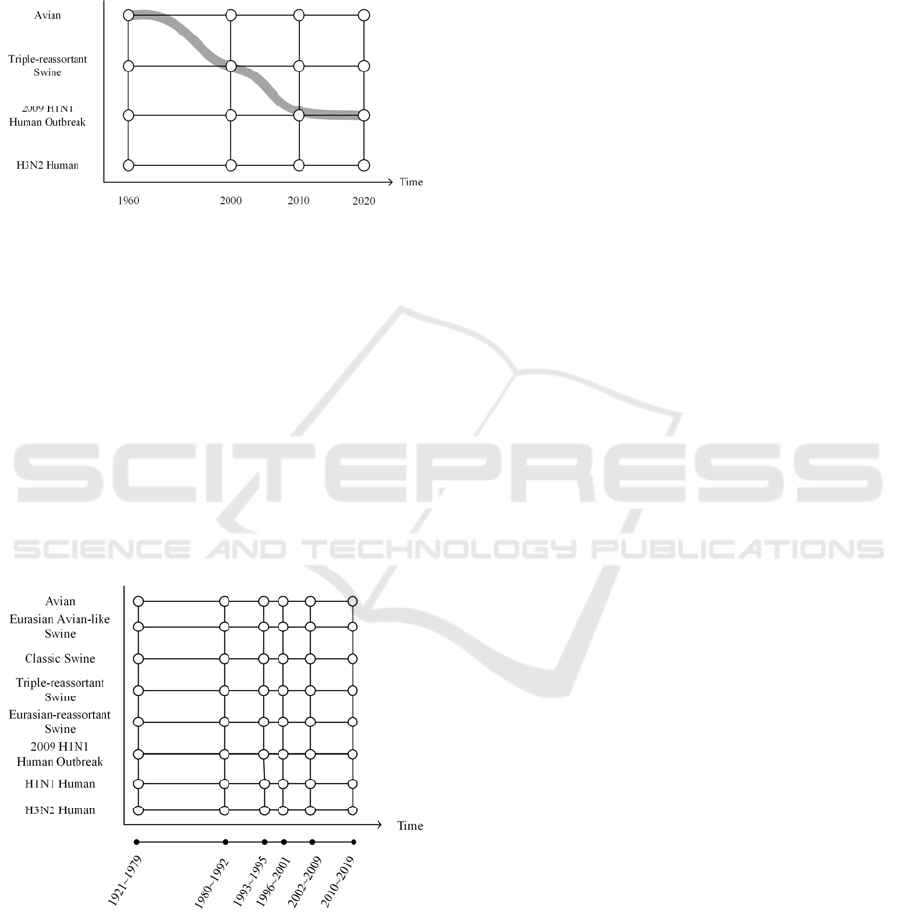
This evolutionary trajectory in Figure 1 shows that

the wild type protein started first as a segment in an

avian virus strain. It then went through the

reassortment events caused by cross-species

mutations, and finally evolved into a segment in the

2009 S-OIV human pandemic virus.

Figure 1: A sample evolutionary trajectory.

2.1 Construction of Evolutionary Grids

A simulated evolutionary trajectory is produced by a

stochastic process that is controlled within the grid. A

node in a grid, as shown in Figure 1, represents a

cluster of proteins that have high similarities

according to some metric, such as sequence

similarity, temporal, or geographical distributions, etc.

Different designs of evolutionary grids, such as the

number of nodes, the members in a node, and the time

interval between nodes, exert different influences

over the stochastic simulation process, which

warrants its flexibility.

Figure 2: A sample design of an evolutionary grid.

To construct an evolutionary grid, we first

determine the types of viruses to study and the

intervals on the time line to set up the framework of a

grid. Figure 2 shows a grid designed for the study of

viruses of various host species, e.g. classic swine. The

time line is divided into six intervals, e.g. 1921~1979.

After the framework of a grid is determined, to

complete the construction is to create the protein

clusters for the nodes on the grid. These clusters

together with the grid framework control the

stochastic simulation.

We first constructed a phylogenetic tree for the

IAV sequences downloaded from NCBI and GISAID

EpiFlu. Based on the phylogenetic analyses (Smith et

al., 2009) of human, swine and avian sample sets, we

assigned these sampled sequences (287 human, 115

swine and 411 avian) as the seeds to the appropriate

clusters according to their isolation years and

subtypes. For example, A PB1 protein

36_H1N1_Swine_swine_ohio_23_1935 in this case

was assigned to the node located at X-coordinate=

“1921~1979” and Y-coordinate= “classic swine” as

shown in Figure 2. Based on the locations of these

seeds in the phylogenic tree, we identified from the

phylogenic tree the lowest common ancestor (LCA)

per host species and subtype. For each LCA in

ascending order of its distance to the root, we

iteratively assigned the remaining sequences under

the LCA to the corresponding cluster on the grid. The

coordinate on the Y-axis was determined by the

LCA’s host species or subtype, and the isolation year

determined the coordinate on the X-axis. We

illustrate the process of host species assignment in

Figure 3 with an example of 10 seed sequences and 7

others. We start with Avian LCA, which is the closest

to the root. All sequences under the LCA except the

seeds are assigned to Avian, including the left-most

sequence in the tree. We next assign the remaining

sequences under Human LCA to H3N2 Human.

Finally, we process those non-seed sequences under

Swine LCA. Note the left-most sequence in the tree

is then reassigned to Swine from Avian. The final

host species assignments are presented at the bottom

of the tree, as shown in Figure 3, and their coordinates

on the timescale X-axis are determined by the

isolation years. We postprocess the clusters by

removing sequences with amino acid similarity

exceeding a certain threshold (set to 0.99) using CD-

HIT (Li & Godzik, 2006).

2.2 Grid-based Stochastic Simulation

We conduct a stochastic process in the sequence-

based space to simulate a point mutation that is

constrained by an evolutionary grid. By performing a

series of stochastic processes to simulate the

accumulation of point mutations, we can generate a

simulated evolutionary trajectory for a wild type IAV

protein.

BIOINFORMATICS 2020 - 11th International Conference on Bioinformatics Models, Methods and Algorithms

110

Figure 3: A sample process of host species assignment. The

seed sequences are denoted by a symbol within the vertical

bars, e.g. the 2

×(Classic Swine) to the left. The others

are the remaining sequences to be assigned to a host species.

2.2.1 Point Mutation and Adaptive Walks

The adaptive walk and mutation landscape models

(Gillespie, 1991; Orr, 2003, 2006) assume that a

current wild-type sequence represents a local

optimum. After an environment change, the fitness of

this wild-type sequence drops, and its adaption is

required. A wild type IAV sequence of L amino acids

has 19L one-point mutants. To complete a beneficial

point mutation in adaption, one favorable mutant

sequence is stochastically selected based on the

fitness, and substituted for the current wild type.

The fitness is assigned to each one-point mutant

in two steps. First, for a given wild-type sequence, we

form a neighborhood of k nearest neighbors according

to sequence similarity. The details of constructing a

neighborhood is described in the next section. We

compute the average sequence similarity between the

k-nearest neighbors and each of the 19L one-point

mutants. Second, we generate and sort 19L+1 random

fitnesses based on a specified probability distribution

(e.g. normal, Gamma or exponential). The i

value is

reserved for the current wild type, where i can be set

to 10, 50 or 150 as in (Orr, 2002), and the remaining

sorted 19L values are assigned to the 19L one-point

mutants individually in descending order of sequence

similarity computed earlier. The 1

to the (i-1)

one-

point mutants in the sorted list are considered the

beneficial mutants as they have higher fitness than the

current wild type. Figure 4 illustrates the process of

fitness assignment.

After the assignment of the fitnesses is complete,

we calculate the mutation probability P

that the

current wild type (i.e. the i

sequence) mutates to the

one-point mutant (t = 1 ~ i-1) in the sorted list. We

define the probability P

as follows.

Figure 4: Fitness assignment.























⋯





(1)





1





(2)















1



,where  1…1 (3)

where F

is the fitness of the r

one-point mutant

sequence, S

is the selection coefficient of the m

one-point mutant sequence, and



is the probability

of fixation for the m

one-point mutant sequence, as

defined in Orr (Orr, 2002) and Gillespie (Gillespie,

1983). We select one of the beneficial mutants

randomly as the next wild-type sequence based on the

probability distribution of P

to implement a

stochastic point mutation. The fitness of the next wild

type (i.e. j

mutant as in Fig. 4) becomes the stopping

threshold for the next point mutation in an adaptive

walk. To check if one-point mutation should continue,

we generate a new set of 19L+1 random fitnesses. If

the current threshold is higher than all the fitnesses, it

indicates a convergence and we stop point mutation;

otherwise, we repeat the same point mutation process

as above. When a new wild type is fitter than all its

one-point mutants, an adaptive walk is complete, and

the fixation of the fittest wild-type sequence

represents a local optimum. This status remains until

the environment changes again. It will then trigger a

new adaptive walk, and the evolution continues. All

these adaptive walks connected together form a

simulated evolutionary trajectory of the initial wild

type.

Unlike previous works that focused on mutational

landscapes, adaption patterns and fitness distributions

(Gillespie, 1991; Orr, 2002; Orr, 2006), our study of

adaption considers sequence similarity, which

enables us to describe the accumulation of point

mutations along a simulated evolutionary trajectory.

Figure 5 shows the process of an adaptive walk.

A Grid-based Simulation Model for the Evolution of Inﬂuenza A Viruses

111

Figure 5: Process of an adaptive walk.

2.2.2 K-nearest-neighbor Neighborhood

As mentioned in the previous section, we sort the 19L

one-point mutants according to their sequence

similarities to a neighbourhood of k-nearest neighbors.

Because the ranking of the mutants is crucial to the

result of point mutation, the members in the

neighborhood consequently play an important role in

the control of adaptive walks.

Figure 6: Construction of neighbourhood for retrospective

simulation. The triangle denotes the initial wild type

isolated in 1978. The shaded area represents a forward k-

nearest-neighbor neighborhood.

We classify the simulated evolutionary

trajectories into two types: retrospective and

prospective. A retrospective trajectory describes the

events of point mutation that may have occurred to a

given wild type. By contrast, a prospective trajectory

predicts the events of point mutation that may occur

in the near future to some current wild type. The k-

nearest-neighbor neighborhood is therefore

constructed differently for retrospective and

prospective simulations.

For retrospective simulation, we construct a

neighborhood from the sequences available on the

evolutionary grid. Given a wild-type sequence, we

first identify its closest mapping sequence on the grid.

For this closest sequence, to form a neighborhood we

locate its k-nearest neighbors on the grid that were

isolated in the same year or later to warrant the

adaptive walk will move forward in time. We call

these neighbors “forward neighbors.”

Figure 7: Construction of neighbourhood for prospective

simulation. The triangle denotes the wild type of interest

isolated in 2010. The irregular shaded area to the left

represents a backward k-nearest-neighbor neighborhood.

The middle rectangular shaded area indicates a pool from

which to create a pseudoneighborhood. The irregular

shaded area to the right shows a k-nearest-neighbor

pseudoneighborhood.

Unlike retrospective simulation, it is not

appropriate to construct a neighborhood directly from

the sequences available on the grid because they were

isolated in the past, and they may mislead the

adaptive walk backward in time. To resolve the

problem with unavailability of forward neighbors, we

create pseudoneighbors. For a current wild type of

interest, we select a sequence available on the grid as

an initial wild type, and run retrospective simulation

multiple times until the simulated evolution reaches

the given wild type of interest or some similar

sequence. If the retrospective evolution cannot reach

the given wild type or even a similar sequence, we

start with a different initial wild type and repeat the

retrospective simulation. We collect the amino acid

mutation frequencies from the retrospective

trajectories, and estimate the first-order and second-

order transition probabilities of amino acids, P(AA

’ |

) and P(AA

’ | AA

i-1

), where AA is an old

BIOINFORMATICS 2020 - 11th International Conference on Bioinformatics Models, Methods and Algorithms

112

amino acid, AA’ is the new amino acid after point

mutation, and i is the position of the amino acid in the

sequence.

In contrast to the k-nearest-neighbor

neighborhood identified in retrospective simulation,

to create a pseudoneighborhood for a wild type of

interest, we first identify its k-nearest sequences that

are available on the grid and were isolated in the same

year or earlier than this wild type. We call these

neighbors “backward neighbors.” From each

backward neighbor sequence, we generate multiple

pseudosequences based on the first-order and second-

order transition probabilities, and collect them into a

pool. Subsequently, we select from the pool the k-

nearest pseudosequences to the wild type to construct

the pseudoneighborhood. Figures 6 and 7 illustrate

the construction of neighborhoods for retrospective

and prospective simulation, respectively.

3 RESULTS AND DISCUSSION

We tested the proposed simulation model on three

internal proteins, PB1, PB2, and NP, of IAVs. For

each protein, we selected four different strains and

tested them in retrospective and prospective

simulations, respectively. Table 1 lists the protein

strains in the study.

Table 1: List of protein strains for simulation tests.

Internal

Protein

(Host)

Strain Name

(retrospective simulation)

Strain Name

(prospective simulation)

PB1

(Human)

A/nt/60/1968

A/England/878/1969

A/Memphis/101/1972

A/England/1972

A/Waikato/16/2000

A/New South Wales/36/2000

A/Queensland/6/2000

A/Western Australia/12/2000

PB2

(Avian)

A/pintail duck/ALB/219/1977

A/mallard/Alberta/46/1977

A/duck/Alberta/35/1976

A/mallard/Wisconsin/524/1979

A/duck/NJ/7717-70/1995

A/mallard/Minnesota/282/2000

A/common teal/Netherlands/10/2000

A/shorebird/Delaware Bay/280/1999

(Swine)

A/swine/Italy/2/1979

A/swine/Wisconsin/1/1967

A/swine/Tennessee/19/1976

A/swine/Illinois/1/1975

A/swine/Wisconsin/125/97

A/swine/Wisconsin/464/98

A/Swine/Iowa/533/99

A/swine/North Carolina/47834/2000

For both retrospective and prospective

simulations, we set the isolation year of the strain as

the start year, and 2018 as the end year. The

simulation model was evaluated from two

perspectives on the evolutionary trajectories. One was

the interspecies-transition pathway on a timescale;

the other was the mutation on IAV genomic

signatures. Unlike conventional phylogenetic tree

analyses, a simulated evolutionary trajectory of an

IAV is able to show when an interspecies transition

may have occurred or will occur, and what the

mutations on the amino acids are.

3.1 Analysis of Interspecies Transitions

We conducted the analysis differently according to

the type of evolutionary trajectories, retrospective or

prospective.

(a)

(b)

(c)

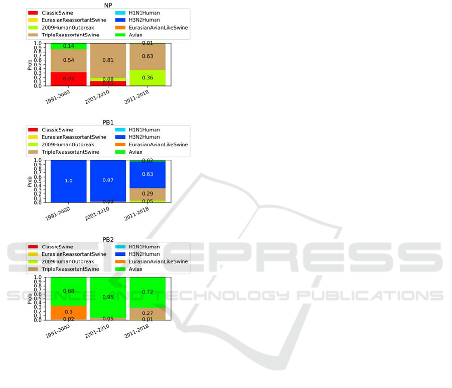
Figure 8: Retrospective evolutionary pathways. (a) NP, (b)

PB1 and (c) PB2.

Each retrospective simulation started with the

isolation year of the selected protein strain, and was

aborted when it reached the year 2018. For each

protein strain, we repeated the same simulation 10

times, and visualized the stochastic evolutionary

pathways in Figure 8. We divided the timescale into

intervals. The height of a rectangular bar in different

colors represents the probability of a host species (and

subtype) for a protein mutant within an interval. For

example, in Figure 8(a) during 2011-2018 the

probabilities of the host species, swine

(TripleReassortantSwine) and human

(2009HumanOutbreak), for an NP protein mutant are

0.05 and 0.95, respectively. We estimated the

probabilities from the ten simulated evolutionary

pathways. For each NP mutant during 2011-2018 on

the 10 evolutionary pathways, we first identified q (q

set to 40 in this study) real NP protein sequences

isolated during 2011-2018 from NCBI and GISAID

EpiFlu that are most similar to this mutant. We

subsequently derived the host species probabilities

A Grid-based Simulation Model for the Evolution of Inﬂuenza A Viruses

113

for an NP mutant from the proportions of these top-q

real sequences according to their host species and

subtypes.

(a)

(b)

(c)

Figure 9: Prospective evolutionary pathways. (a) NP, (b)

PB1 and (c) PB2.

We noted a marked rise in the probability of

TripleReassortantSwine during 1991-2000 for NP

proteins (28%), as shown in Figure 8(a). In addition,

the probability of 2009HumanOutbreak increased to

28% during 2001-2010, and reached 95% in the final

interval. Our simulation results of interspecies

transitions were consistent with the previous study

that the reassortment events may have occurred

during 1990-2001 and led to the human pandemic in

2009 (Smith et al., 2009). By contrast, Figure 8(b)

and (c) show that the probabilities of

TripleReassortantSwine during 1991-2000 were

infinitesimal for PB1 (< 1%) and PB2 (2%). Not until

the final two intervals, 2001-2010 and 2011-2018, did

the probabilities of TripleReassortantSwine and

2009HumanOutbreak become noticeable. These

discrepancies may be attributable to the genetic

variabilities in internal proteins that our simulation

failed to address due to the small number of protein

strains in our current study.

To evaluate the predictive performance of

prospective simulations, we selected protein strains

isolated during 1995-2000. For each strain, we first

conducted 10 retrospective simulations to estimate

the transition probabilities of amino acids from the

evolutionary trajectories. For each strain we

simulated 10 prospective pathways starting from its

isolation year to 2018 based on the estimated

transition probabilities. Note that the construction of

the prospective pathways for a protein strain did not

depend on any other real strains available but isolated

later than the strain in test. Therefore, these

prospective pathways were considered the

predictions about this protein strain, and their validity

could be verified by previous studies of IAVs. For

example, a simulated prospective pathway of

A/Waikato/16/2000 provides a prediction of its

potential interspecies transitions after 2000. We

summarize the results in Figure 9.

Similar to the results of the retrospective

simulations in Figure 8(a), Figure 9(a) shows the

highest probability of TripleReassortantSwine for NP

proteins during 1991-2000 and 2001-2010 in the

prospective simulations. The probability of

2009HumanOutbreak started to increase during

2001-2010, and became more evident during 2011-

2018, which was in accordance with the temporal

reconstruction of the reassortment history of the 2009

human pandemic (Smith et al., 2009). We also

observed from Figure 9(b) that the first reassortment

of swine lineages with PB1 proteins occurred during

2001-2010. The predicted interval agreed well with

the previous finding that a new triple reassortant

swine virus was first detected in 1998 (Brown et al.,

1998). In comparison with Figure 8(c), Figure 9(c)

shows similar probability distributions of the host

species during 1991-2000. While the interspecies

transition to 2009HumanOutbreak did not occur until

2011-2018, and the probability was small (1%), as

shown in Figure 9(c), the predicted interval was close

to when the outbreak occurred.

3.2 Analysis of Mutation on Genomic

Signatures

The establishment of an influenza virus in a new host

is rare because it requires the efficient and effective

transmission, replication, and adaptation of the virus.

Nevertheless, pandemics caused by widely

circulating viruses with the potential to transmit to

humans remain a threat (Naffakh et al., 2008). Unlike

BIOINFORMATICS 2020 - 11th International Conference on Bioinformatics Models, Methods and Algorithms

114

the analysis of molecular mechanisms, using in vitro

systems and reverse genetics of influenza viruses, the

analysis of a continuously increasing amount of

available viral sequence data enables a cost-effective

approach for the identification of genomic signatures

as host-range determinants (Hu et al., 2014).

Genomic signatures can change because of point

mutations and interspecies reassortment. The

simulation model could provide a deeper insight into

the transitions of these signatures, and increase our

understanding of the adaption trends.

Table 2: Results of genomic signature mutations based on

retrospective evolutionary trajectory analysis. (a) NP, (b)

PB1 and (c) PB2.

(a)

NP

Swine



Human

Interval

position

AA

mutation

1961

|

1970

1971

|

1980

1981

|

1990

1991

|

2000

2001

|

2010

2011

|

2018

313

F→V 0 0 0 0 17 70

F→Y 0 0 0 0 0 1

109 I→V 0 0 0 0 0 100

217 I→V 0 0 0 23 68 219

353 V→I 0 0 0 63 24 10

(b)

PB1

Swine



Human

Interval

position

AA

mutation

1961

|

1970

1971

|

1980

1981

|

1990

1991

|

2000

2001

|

2010

2011

|

2018

327 R→K 1 25 8 108 331 4

(c)

PB2

Avian



Human

Interval

position

AA

mutation

1961

|

1970

1971

|

1980

1981

|

1990

1991

|

2000

2001

|

2010

2011

|

2018

271 T→A 0 0 0 72 61 2

588 A→T 0 0 0 87 74 2

684 A→S 0 0 0 0 29 16

453 P→S 0 0 0 0 32 36

292

I→V 0 2 16 61 55 59

I→T 0 0 0 0 0 3

475 L→M 0 0 14 54 1 31

559 T→I 0 0 0 0 26 7

590 G→S 0 0 0 0 53 1

We examined the retrospective and prospective

evolutionary trajectories for the mutations on the

host-associated signatures that have been identified in

previous studies (Miotto et al., 2010; Hu et al., 2014;

Pan et al., 2009). Seventeen and one amino acid

signatures have been identified on NP and PB1

proteins, respectively, to separate swine influenza

viruses from human influenza viruses. Twenty amino

acid signatures have been found on PB2 proteins to

distinguish avian influenza viruses from human

influenza viruses.

Table 3: Results of genomic signature mutations based on

prospective evolutionary trajectory analysis. (a) NP, (b)

PB1 and (c) PB2.

(a)

NP

Swine



Human

Interval

position

AA

mutation

1991

|

2000

2001

|

2010

2011



2018

109 I→V 0 10 2

217 I→V 0 3 3

353

V→I 10 29 9

V→S 0 0 4

344 S→L 0 0 1

(b)

PB1

Swine



Human

Interval

position

AA

mutation

1991

|

2000

2001

|

2010

2011

|

2018

327 R→K 2 76 74

(c)

PB2

Avian



Human



Interval

position

AA

mutation

1991

|

2000

2001

|

2010

2011

|

2018

271 T→A 0 2 9

292

I→V 99 132 48

I→T 6 10 3

475 L→M 83 72 29

368 R→K 0 1 0

613 V→T 7 24 30

199 A→S 0 1 2

674 A→T 0 0 2

702 K→R 5 50 31

44 A→S 0 1 3

661 A→T 0 2 1

We checked each host-associated signature on

NP, PB1 and PB2 along the simulated evolutionary

trajectories, retrospective and prospective,

respectively. From all the simulated trajectories, we

recorded the frequency of signature mutations within

each time interval. We identified from the

retrospective trajectories 4 NP signatures, 8 PB2

signatures, and the one PB1 signature. In addition, we

also identified 4 NP signatures, 10 PB2 signatures,

and the same PB1 signature from the prospective

trajectories. They all showed at least one mutation at

some time on the evolutionary trajectories, and

different frequencies of mutations in different

intervals. We summarize the results in Tables 2 and

3. For example, Table 2(a) shows that on all the

simulated retrospective trajectories of NP, 17

occurrences of amino acid mutation from F to V were

identified during 2001-2010.

By comparing Table 2 with Table 3, we observed

that most of the signature mutations identified from

the prospective trajectories were coincident with

those identified from the retrospective trajectories.

Three out of four NP signatures found from the

prospective trajectories were also identified from the

A Grid-based Simulation Model for the Evolution of Inﬂuenza A Viruses

115

retrospective trajectories. The only PB1 signature

mutation, PB1-R327K, separating swine viruses from

human viruses was found from both the retrospective

and prospective trajectories. Three PB2 signatures

were also identified from both the retrospective and

prospective trajectories. These findings suggest that

the predicted evolutionary trajectories produced by

prospective simulations are rather consistent with the

retrospective evolutionary trajectories. Furthermore,

it is noteworthy that there was a marked rise in the

frequency of mutations on the signatures during

1990-2000 and 2001-2010, as shown in Tables 2 and

3, which was consistent with the time when the triple

reassortment events occurred.

4 CONCLUSIONS

We proposed a grid-based simulation model to

analyze and predict the evolutionary trends of IAVs.

Unlike previous approaches based on phylogenetic

trees or complex dynamics models, the proposed

simulation model only involves a series of adaptive

walks controlled by stochastic point mutations

constrained within an evolutionary grid. The

experiments of both interspecies transitions and

genomic signature mutations have demonstrated

promising results. It warrants further investigation

into the applicability of the simulation model for

predicting the evolutionary trends of IAVs.

ACKNOWLEDGEMENTS

The research was partially supported by Ministry of

Science and Technology of Taiwan (MOST 108-

2221-E-009-086).

REFERENCES

Brown, I. H., Harris, P. A., McCauley, J. W., Alexander,

D.J., 1998. Multiple genetic reassortment of avian and

human influenza A viruses in European pigs, resulting

in the emergence of an H1N2 virus of novel genotype.

J. Gen. Virol. 79, pp. 2947–2955.

Gerrish, P., 2001. The rhythm of microbial adaptation.

Nature, vol. 413, pp. 299–302.

Gillespie, J. H., 1983. A simple stochastic gene substitution

process. Theor. Popul. Biol. 23:202–215.

Gillespie, J. H., 1991. The causes of molecular evolution.

Oxford Univ. Press, Oxford, U.K.

Hu, Y., Tu, P., Lin, C., Guo, S., 2014. Identification and

Chronological Analysis of Genomic Signatures in

Influenza A Viruses. Plos ONE, 9(1), e84638.

Lässig, M., Łuksza, M., 2014. Adaptive Revolution: Can

we read the future from a tree. eLife Sci., 3, e05060.

Li, W., Godzik, A., 2006. Cd-hit: a fast program for

clustering and comparing large sets of protein or

nucleotide sequences. Bioinformatics, vol. 22(13), pp.

1658–1659.

Łuksza, M., Lässig, M., 2014. A Predictive Fitness Model

for Influenza. Nature, 507, pp. 57–61.

Miotto, O., Heiny, A. T., Albrecht, R., Garcı´a-Sastre, A.,

Tan, T.W., et al., 2010. Complete-Proteome Mapping

of Human Influenza A Adaptive Mutations:

Implications for Human Transmissibility of Zoonotic

Strains. PLoS ONE 5(2): e9025.

Naffakh, N., Tomoiu, A., Rameix-Welti, M-A, van der

Werf, S., 2008. Host Restriction of Avian Influenza

Viruses at the Level of the Ribonucleoproteins. Annu.

Rev. Microbiol 62: 403-424.

Neverov, A. D., Kryazhimskiy, S., Plotkin, J. B., Bazykin,

G. A., 2015. Coordinated Evolution of Influenza A

Surface Proteins. PLoS Genetics, 11(8), e1005404.

Orr, H. A., 2002. The distribution of fitness effects among

beneficial mutations. Genetics, vol. 163, pp. 1519–

1526.

Orr, H. A., 2002. The population genetics of adaptation: the

adaption of DNA sequences. Evolution, 56(7), pp.

1317–1330.

Orr, H. A., 2006. The population genetics of adaptation on

correlated fitness landscapes: the block model.

Evolution, 60(6), pp. 1113–1124.

Pan, C., Cheung, B., Tan, S., Li, C., Li, L., et al., 2010.

Genomic Signature and Mutation Trend Analysis of

Pandemic (H1N1) 2009 Influenza A Virus. PLoS ONE

5(3): e9549.

Perelson, A. S., Macken., C. A., 1995. Protein evolution on

partially correlated landscapes. Proc. Natl. Acad. Sci.

USA 92, pp. 9657–9661.

Smith, G. J. D. et al., 2009. Origins and evolutionary

genomics of the 2009 swine-origin H1N1 influenza A

epidemic. Nature, Vol. 459, pp. 1122–1126.

Timofeeva, T. A., Asatryan, M. N., Altstein, A. D.,

Narodisky, B. S., Gintsburg, A. L., Kaverin, N. V.,

2017. Predicting the Evolutionary Variability of the

Influenza A Virus. ACTA NATURAE, Vol. 9, No.

3(34), pp. 48–54.

BIOINFORMATICS 2020 - 11th International Conference on Bioinformatics Models, Methods and Algorithms

116