Automatic Detection of Epileptic Spikes in Intracerebral EEG with

Convolutional Kernel Density Estimation

Ludovic Gardy

1,2,3 a

, Emmanuel J. Barbeau

1,2 b

and Christophe Hurter

3 c

University of Toulouse, UPS, Centre de Recherche Cerveau et Cognition, Toulouse, France

CNRS, CerCo, Purpan Hospital, Toulouse, France

French Civil Aviation University, ENAC, Avenue Edouard Belin, Toulouse, France

Keywords:

Electroencephalography, EEG, Time Series Visualization, Signal Processing, Kernel Density Estimation,

Convolution, Noisy Signal, Event Detection, Epilepsy, Accessibility.

Abstract:

Analyzing the electroencephalographic (EEG) signal of epileptic patients as part of their diagnosis is a very

long and tedious operation. The most common technique used by medical teams is to visualize the raw signal

in order to ﬁnd pathological events such as interictal epileptic spikes (IESs) or abnormal oscillations. More and

more efforts are being adopted to try to facilitate the work of doctors by automating this process. Our goal was

to analyze signal density ﬁelds to improve the visualization and automatic detection of pathological events. We

transformed the EEG signal into images on which we applied a convolution ﬁlter based on a Kernel Density

Estimation (KDE). This method that we propose to call CKDE for Convolutional Kernel Density Estimation

allowed the emergence of local density ﬁelds leading to a better visualization as well as automatic detection

of IESs. Future work will be necessary to make this technique more efﬁcient, but preliminary results are very

encouraging and show a high performance compared to a visual inspection of the data or some other automatic

detection techniques.

1 INTRODUCTION

Epilepsy is the name of a brain disorder character-

ized predominantly by recurrent and unpredictable in-

terruptions of normal brain function, called epileptic

seizures (Fisher et al., 2005). Treating this disease

sometimes requires the patient to undergo a record of

his brain activity by Electroencephalography (EEG)

in order to characterize the epileptogenic network,

i.e., the brain area(s) involved in the seizures. EEG

results from the electric signal generated by the co-

operative action of brain cells (Blinowska and Durka,

2006). When epilepsy is drug-resistant, the solution

to cure the patient is to surgically remove the area

of his brain that causes seizures. To locate this area,

it is often necessary to go through a stereoelectroen-

cephalography (SEEG) consisting of the deep intrac-

erebral implantation of electrodes. The depth EEG

of the patient is recorded 24 hours a day for 6 to

15 days and then examined later by epileptologists.

The electrophysiological markers and criteria for de-

https://orcid.org/0000-0002-2977-8831

https://orcid.org/0000-0003-0836-3538

https://orcid.org/0000-0003-4318-6717

termining whether a cerebral area is impaired are still

being deﬁned (Valero et al., 2017; Roehri et al., 2017;

Frauscher et al., 2017; Roehri et al., 2018). How-

ever, some markers such as interictal epileptic spikes

(IESs) are characteristic of the epileptogenic network

(Talairach and Bancaud, 1966). They appear sponta-

neously between periods of seizures and are of high

amplitude for a duration ranging from 30 to 100 mil-

liseconds (De Curtis and Avanzini, 2001) followed by

a slow component for around 150 to 200 millisec-

onds (Staley and Dudek, 2006). IESs are generated

by synchronous discharges of a group of neurons in a

region referred to as the irritative zone (Latka et al.,

2003). While some would argue that the neural net-

work that produces IESs is not always identical to the

seizure onset zone, IESs are useful to support the di-

agnosis of epilepsy (Staley and Dudek, 2006). Other

markers, more recent and not used in clinical practice

yet such as fast-ripples, are being studied by several

teams around the world and could be essential mark-

ers of the seizure onset zone (Staba et al., 2002; Ibarz

et al., 2010). There is currently no ofﬁcial tool that

can be used in clinical practice to detect these dis-

crete and transient events, such as IES or fast-ripples.

Gardy, L., Barbeau, E. and Hurter, C.

Automatic Detection of Epileptic Spikes in Intracerebral EEG with Convolutional Kernel Density Estimation.

DOI: 10.5220/0008877601010109

In Proceedings of the 15th International Joint Conference on Computer Vision, Imaging and Computer Graphics Theory and Applications (VISIGRAPP 2020) - Volume 2: HUCAPP, pages

101-109

ISBN: 978-989-758-402-2; ISSN: 2184-4321

101

Moreover, their characteristics can differ from one pa-

tient to another and vary in shape, duration, or fre-

quency, making them very difﬁcult to detect by an au-

tomatic tool. Many attempts have been made to create

such devices, but they’ve had a relatively low impact

and have not passed the gates of research laboratories.

However, we address that question with a completely

new approach that could provide an efﬁcient solution.

The amounts of data to be analyzed are so huge; we

estimate it at around 317 billions of electrophysiolog-

ical values for a 15-day, or 360 hours, recording in

one patient. We can no longer let clinicians manu-

ally look at the signal and search inside for patho-

logical events without help. The technique we pro-

pose to visualize and automatically tag pathological

events in this massive amount of noisy EEG signal

is based on image processing. Our tests show that

IESs have a particular signature in the ﬁeld of densi-

ties. We transformed the signal into an image using

Kernel Density Estimation (Silverman, 2018) and ap-

plied a convolution onto this image to build density

ﬁelds based on the spacing of pixels. The brief and

rapid amplitude changes during spikes lead to a larger

gap between activated pixels which is characterized

by a low density after convolution. These low densi-

ties are the ones that can be visualized and even au-

tomatically recorded. We analyzed the intracerebral

EEG recordings of a patient treated in the epilepsy

department of CHU Purpan in Toulouse, France. Our

method allowed us to obtain an improved visualiza-

tion of the EEG signal enabling a fast localization of

the IESs but also automatic detection of these patho-

logical events. There is still much effort to be made

to generalize this approach and make it functional for

clinical implications, but the preliminary results we

obtain using it are very encouraging. In this paper, we

will deﬁne epilepsy and diagnostic problems before

presenting the related works about EEG visualization

and automatic pattern detection, then present the re-

sults we have obtained and discuss them.

2 RELATED WORKS

This work builds upon recent studies covering time-

series visualization (Wang et al., 2017) as well as the

automatic search for pathological events such as inter-

ictal epileptic spikes (IESs) in the EEG signal (Roehri

et al., 2018). The question of IESs as markers of the

epileptogenic network has been widely studied, but no

study has yet made it easier to visualize them or de-

tect them automatically. These techniques are either

not reliable enough or too long or difﬁcult to use.

2.1 EEG Visualization

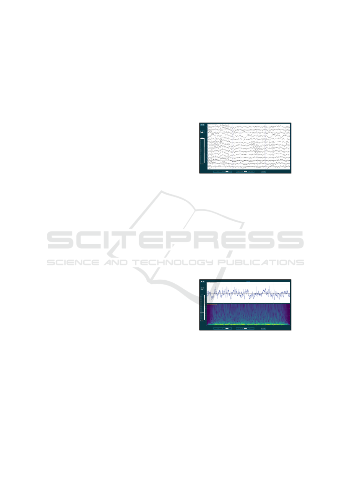
EEG recordings are most of the time represented as

curve-shaped amplitudes varying over time (ﬁgure 1).

These line graphs are a quick and easy way to describe

and understand brain activity. Clinicians and neurol-

ogists, in particular, are very attached to this visual-

ization because they are used to it and understand it

well.

Figure 1: Classical representation as a line graph of an EEG

signal. Each line represents a channel from an intracerebral

recording.

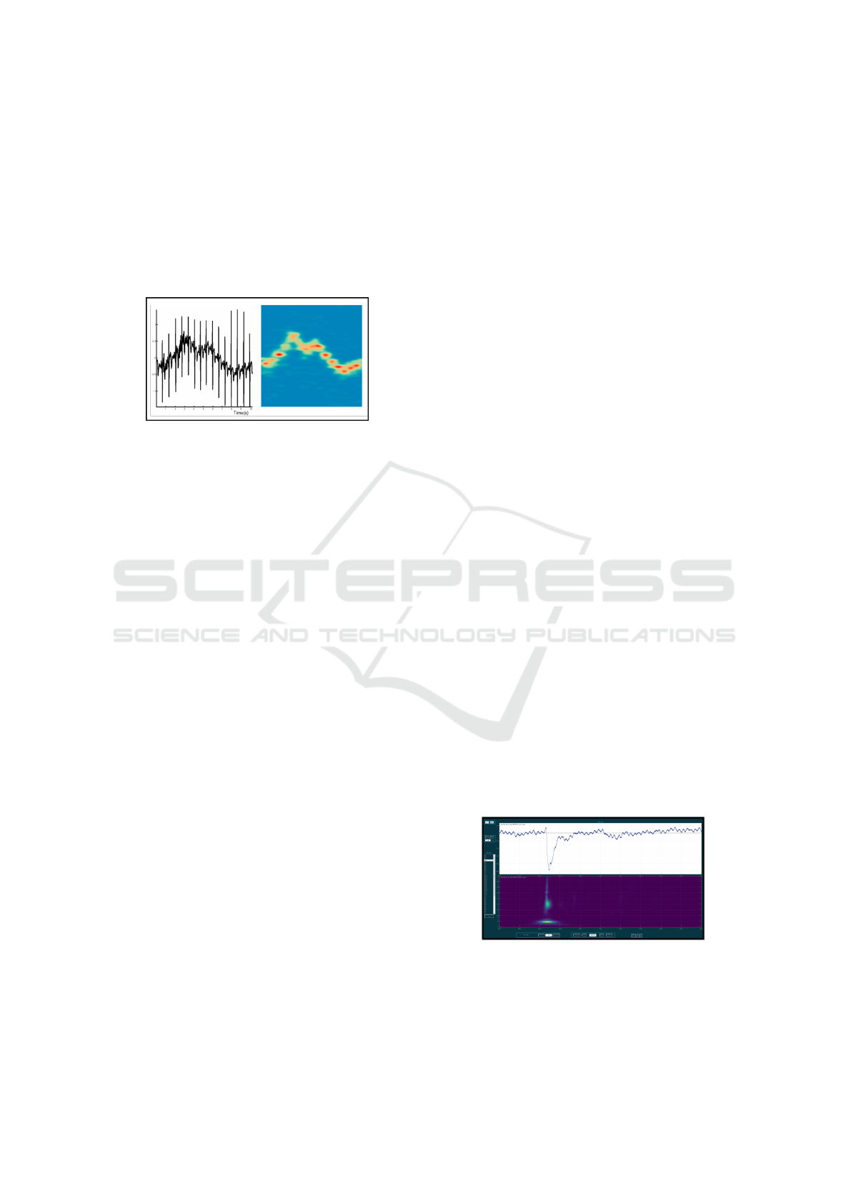
Time-frequency representation (ﬁgure 2) is an-

other way to display the signal, seldom used in clini-

cal practice but appreciated by neuroscientists. The

frequency spectrum is a good indicator of ongoing

cognitive processes and possibly epileptic events such

as pathological oscillations (Bragin et al., 2002; Bra-

gin et al., 1999a; H

oller et al., 2015). The promising

results of a time-frequency analysis of intracerebral

EEG signals in epilepsy will probably make this a not

to be missed step soon from a medical point of view

as well.

Figure 2: Additional time-frequency representation for one

channel. Top graph: raw data, bottom graph: the frequency

values are represented along the y-axis and the power in

these frequencies on a color scale.

2.2 Time Series Visualization

Many variants of time series representations have

been proposed to synthesize or improve visualiza-

tion (Saito et al., 2005; Javed and Elmqvist, 2010;

Van Wijk and Van Selow, 1999; Weber et al., 2001;

Lin et al., 2004; Kincaid and Lam, 2006; Hao et al.,

2007; Zhao et al., 2011) but their effectiveness has

been discussed, and the classical representation is still

HUCAPP 2020 - 4th International Conference on Human Computer Interaction Theory and Applications

102

favored in practice. However, a recent study (Wang

et al., 2017) proposed the application of Kernel Den-

sity Estimation (KDE) to transform a signal into a

density ﬁeld (ﬁgure 3). They showed that it leads to

a new type of signal, and in some cases, the visual-

ization is improved compared to the original one. We

think that the visual aspect is not the only one to be

interesting, but that the whole notion of signal density

is.

Figure 3: Density representation of a time series. Figure

from (Wang et al., 2017).

2.3 Event Detection

Manually searching for pathological events such as

interictal epileptic spikes (IESs) in the EEG signal

is a very long and tedious operation for epileptolo-

gists. During the past decades, many methods were

proposed to detect theses events automatically (Birot

et al., 2013; Gotman, 1999). The noise makes it

difﬁcult for an algorithm to be efﬁcient in this task.

Furthermore, nowadays technology and storage ca-

pacities, allowing several days of 24/7 recordings on

more than a hundred channels simultaneously, yield a

considerable amount of data. Some algorithms work

quite fast but are just as much sensitive to noise and

no longer work when the pattern to research differs

from the input signal. Some others are relatively efﬁ-

cient, but the computation time for large amounts of

data is discouraging.

2.3.1 Dynamic Time Warping

In time series analysis, dynamic time warping (DTW)

is one of the algorithms for measuring similarity be-

tween two temporal sequences, for instance, two time

series of the same length (Keogh et al., 2009; Ding

et al., 2008). The difference with a pure Euclidean

Distance is that the whole sequence is taken into ac-

count to calculate the similarity between the pattern

and the input signal, not just the sum of the distances

between each point of the two sequences. DTW has

been used for some biological applications (Rakthan-

manon et al., 2012; Chadwick et al., 2011) or gesture

recognition (Alon et al., 2008; Wobbrock et al., 2007)

but the computation time on a massive amount of data

as well as the difﬁculty to detect an event when the in-

put signal differs from the pattern can make it barely

efﬁcient. An improved version of the Trillion algo-

rithm from the UCR (University of California, River-

side) suite ((Rakthanmanon et al., 2012)) have been

developped and tested (Jing et al., 2016) on a hun-

dred patients, allowing a good recognition of IESs.

Nevertheless, the necessity of having a pattern to re-

search is still a problem. A user still needs to spec-

ify a template, and there is a large variability of spike

waveforms within and between patients among other

factors.

2.3.2 Machine Learning

The past decade has seen the rise of machine learn-

ing in EEG signal processing, giving birth to a rich

literature. Work in this domain has focused as much

on the automatic search for epileptic seizures (Song

et al., 2012) as on that of epileptic markers such as

pathological oscillations or IESs (Jrad et al., 2016;

Birot et al., 2013). Many problems remain, start-

ing with the fact that feature engineering is a time-

consuming and challenging task. Furthermore, pre-

processing and cleaning the EEG signal requires to

manipulate tools that are not easy to use, especially

for clinicians. Deep learning methods have been more

recently built with the promise to overcome these is-

sues or at least lighten them as it can learn good fea-

ture representations from raw data (Roy et al., 2019).

It is essential to follow carefully this area of literature

which is promising but not yet functional in practice.

2.3.3 Time-frequency

As shown in ﬁgure 4, sharp transients events present

in depth-EEG signals (typically, the spike compo-

nent of interictal epileptic spikes - IESs) are associ-

ated with an abrupt increase of the signal energy in

the lower and higher frequency bands (B

enar et al.,

2010).

Figure 4: Example of an interictal epileptic spike (IES) in

a one second time window. Top: raw signal, bottom: time-

frequency representation.

An up-and-coming tool for the automatic detec-

tion of IES and pathological oscillations, based on

Automatic Detection of Epileptic Spikes in Intracerebral EEG with Convolutional Kernel Density Estimation

103

time-frequency analysis, is Delphos (Roehri et al.,

2018; Roehri et al., 2016). However, we believe that

a density analysis of the signal could lead to new pos-

sibilities and compete or cooperate with the existing

techniques in the challenge toward automatic detec-

tion. Many false positives currently make the ex-

ploitation of time-frequency data difﬁcult, while this

2-dimensional signal may beneﬁt from a density anal-

ysis to sort the events detected by a threshold in the

frequency-domain.

3 ESTIMATING DENSITIES

By converting a 1-dimensional EEG signal composed

of a list of ordered values into 2-dimension, we ob-

tain an image, which is an area of pixels. Thus, when

the signal varies in amplitude or frequency, this area

of pixels is affected. Two-dimensional convolution

is a technique commonly used in image processing

to apply effects such as blurring, sharpening, or edge

detection. We used this technique, that affects pix-

els whose value is different from 0, on our EEG sig-

nal to emerge density ﬁelds that could witness the

occurrence of pathological events. Sharp amplitude

variations during IESs have the effect of spacing the

points, and therefore the pixels representing the sig-

nal on the image, from each other. It is this notion of

spacing between points that we can exploit to iden-

tify IESs in EEG. Typically the electrophysiological

changes of the brain signal are gradual and homoge-

neous, but during an IESs they become huge in a short

time. When convolution is applied, non-pathological

variations appear under the form of high densities and

IESs under the form of low density because of the

fast spacing between the points in the same amount

of time.

3.1 Kernel Density Estimation

It was necessary to transform the 1-dimensional EEG

signals into 2-dimensional images in order to apply

a convolution. Using KDE allowed to convert each

value (a ﬂoat or an integer) of the 1-dimensional EEG

signal into a vector representing a Gaussian-shaped

density probability of ﬁnding this value within a range

of values. The aggregation of these vertically trans-

posed vectors along the time axis constitutes a 2-

dimensional image of the original 1-dimensional EEG

signal (ﬁgure 5).

Figure 5: Left: A randomly simulated 1-dimensional sig-

nal where each timestamp is associated with a single value.

Right: The same signal converted into a 2-dimensional im-

age using KDE. Each timestamp is associated with a verti-

cal vector representing a Gaussian-shaped density probabil-

ity.

3.2 Convolution of the Imaged Signal

Convolution consists of applying a kernel on each of

the pixels of the image. This technique has the effect

of modifying the value of the current pixel by consid-

ering the value of the neighboring pixels. Only pixels

with a value different from 0 are affected. This pro-

cess of adding each element of the image to its local

neighbors, weighted by a kernel, leads to an improved

visualization with additional density ﬁeld. Let d

de-

note the pixel value of an image and V its value after

processing, the convolution can be modeled by

V =|

∑

i=1

(

∑

j=1

i j

)

Where:

• f

= the coefﬁcient of a convolution kernel at po-

sition i,j (in the kernel);

• d

= the data value of the pixel that corresponds

to f

;

• q = the dimension of the kernel, assuming a square

kernel (if q = 3, the kernel is 3*3);

• F = either the sum of the coefﬁcients of the kernel

or 1 if the sum of coefﬁcients is 0;

• V = the output pixel value;

The obtained density ﬁeld, looking like an im-

proved color-scaled line graph (ﬁgure 6), is affected

both by variations in the amplitude and frequency of

the original signal. If two pixels of value superior to

0 are side by side, then the two kernels overlap, and

the original pixels are strengthened. If the pixels are

distant, then they are not strengthened by their neigh-

bors. The closer they are to each other, the higher the

local density.

We called Convolutional Kernel Density Estima-

tion (CKDE) the technique we used here, which aims

to transform the time series into images and to apply

a two-dimensional convolution on it.

HUCAPP 2020 - 4th International Conference on Human Computer Interaction Theory and Applications

104

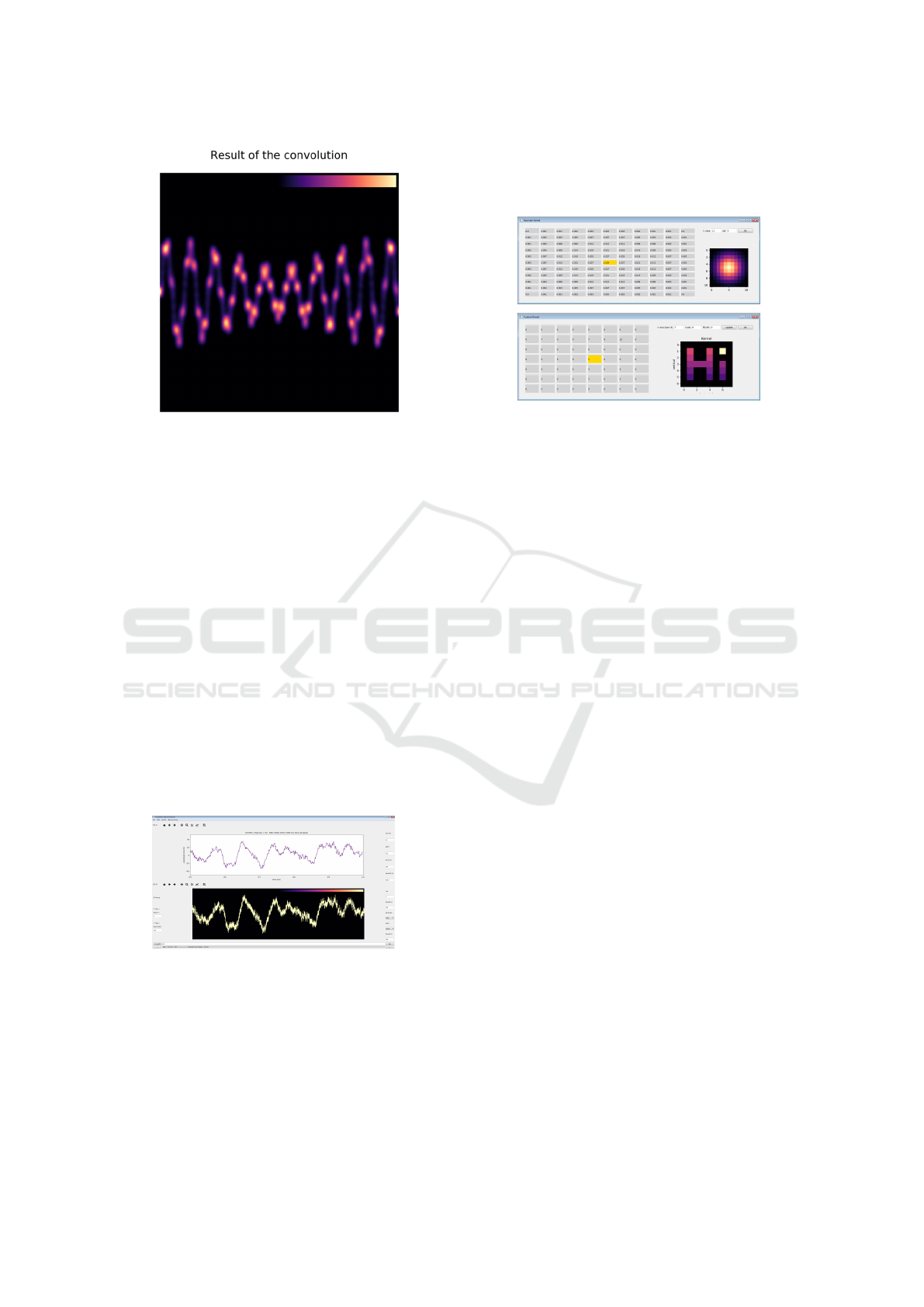
Figure 6: After the application of a Gaussian kernel of size

11 and standard deviation 3 on the image, pixels that are

close to each other are strengthened. On the contrary, pixels

that are distant to each other are barely reinforced.

4 USER INTERFACE

4.1 Implementation

We have built a user interface employing PyQt5 in

Python 3.6 to allow the user to visualize and interact-

ing live with the data. The top panel of the main win-

dow displays the 1-dimensional original signal and

bottom panel the 2-dimensional imaged-signal (ﬁg-

ure 7). Graphical characteristics and window settings

can be modiﬁed by the user using text boxes, combo

boxes, toolbars, and menus on the top and sides of the

window. Some possible actions are, for instance, pan-

ning, zooming, changing colors, moving along the x

and y axes, or saving the ﬁgures.

Figure 7: Main window of the GUI. The two panels at the

center of the main window represent the 1-dimensional and

the 2-dimensional signals. Live interactions are possible

with both.

A user menu is also available for more sophisti-

cated options such as creating a kernel for image con-

volution. Opening the kernel window (ﬁgure 8) al-

lows the user to generate a Gaussian kernel with or

without customizing its parameters (size and standard

deviation). He can alternatively create a wholly cus-

tomized kernel by ﬁlling a grid of the size he wants

the values he wants.

Figure 8: The kernel window allows the setting and drawing

of the kernel that will be employed for image convolution.

Top: Gaussian kernel, bottom: custom kernel.

The user can travel forward or backward in the

time dimension of the signals by using his keyboards’

left or right arrows or those located at the bottom of

the window. Otherwise, it is possible to directly type

a time value in seconds in the text box between the

arrows.

4.2 User Feedback

The only user of the GUI described is the ﬁrst author

of this paper, accustomed to analyzing EEG signals

on different clinical or research software. The GUI

was designed to visualize the original signal and its

associated image to identify possible errors in the al-

gorithm, which is still under development. The main

idea being a proof of concept that density analysis of

EEG can be useful, only one recording channel at a

time is displayed, to avoid missing any important de-

tail (but all channels are processed). Navigation over

time is instantaneous, as is the navigation from one

channel to another or the enabling and disabling of

the convolution, allowing a fast and efﬁcient interac-

tion. An upcoming more sophisticated interface will

be developed soon with the ability to visualize multi-

ple channels at once and a more straightforward de-

sign so that the platform can be used instinctively by

other users.

5 RESULTS

We have evaluated the efﬁciency of EEG signal 2-

dimensional convolution to visualize and automati-

cally detect interictal epileptic spikes (IESs). The data

used are those of a patient who was hospitalized in

2015 and we know well. The EEG signal from the

Automatic Detection of Epileptic Spikes in Intracerebral EEG with Convolutional Kernel Density Estimation

105

same patient were used in a previous study for which

the purpose was different (Despouy et al., 2019). For

this last study, the EEG signal was carefully examined

and tagged. We ran the current tests on a 10 minutes

part of this tagged signal and compared previous man-

ual detection of IESs to automatic detection using our

new method. This data set was composed of a hun-

dred intracerebral macroelectrodes recorded at 2048

Hz that we downsampled at 512 Hz.

5.1 Visualization of Events

The visual inspection of densities (ﬁgure 9) allowed

an easy identiﬁcation of IESs, which are character-

ized by low densities due to the larger spacing be-

tween pixels.

Figure 9: Convolution applied on one channel of the imaged

EEG signal, which appears as a color-scaled line graph. Ex-

ample of density decrease during an IES caused by the sig-

niﬁcant spacing between pixels during this sharp amplitude

changing.

On the previous example, the size of the image

was 512 (horizontal length) * 150 (vertical length),

and the applied kernel was of size 7 * 7 with custom

values, as follows:







9 9 9 9 9 9 9

9 9 9 10 9 9 9

9 9 9 9 9 9 9







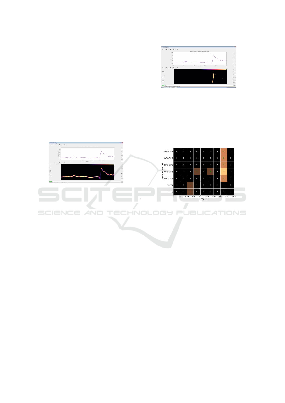
5.2 Automatic Detection of Events

A low pass ﬁlter was applied to the density ﬁeld in

order to remove everything from the image except the

IESs (ﬁgure 10). This means that only the densities

forming the IES are conserved since all the others are

set to 0. The densities resulting from IESs thus be-

come high densities. By summing the densities of

each pixel of the resulting image, we discern if an IES

is present or not. If no IES is present, the total density

Figure 10: Image after application of a low pass ﬁlter. All

the high densities are removed to display only the IESs.

on the image will be around 0. If there is one, it will

be higher, between 400 to more than 1000.

15 IESs were automatically identiﬁed in the por-

tion of the analyzed signal. Among them, 13 were

true IESs, while 2 were false positives (ﬁgure 11).

100% of the events that were tagged during previous

visual inspection were automatically identiﬁed.

Figure 11: Map of detected events. The green text color

indicates the correctly detected IESs, the red color the false

positives. The names of the channels on which an event

has been detected are represented along the y-axis. Time is

represented in seconds along the x-axis. The more events

detected in a given time period, the lighter the square corre-

sponding to this time period for a given recording channel.

An IES is detected when the total density on the

remaining image after removal of high densities by

ﬁltering exceeds a certain threshold. It works well to

detect pathological events but also can lead to false

positives, which are mainly due to two things (ﬁgure

12). Firstly, an accumulation of residual densities ac-

companying rapid micro-changes in signal intensity.

Secondly, an accumulation of low densities related to

the borders of the density ﬁeld not being eliminated

during the ﬁltering. We will expose in the Discussion

a way to solve these problems.

The main objective was to ensure the efﬁciency of

detection. Thus, minimal effort was allocated to in-

crease the speed of computation which currently lasts

90 minutes for a 10 minutes signal. Table 1 summa-

rizes the parameters used for image generation from

the original signal, kernel creation, and convolution,

as well as the characteristics of the automatic detec-

tion process.

HUCAPP 2020 - 4th International Conference on Human Computer Interaction Theory and Applications

106

Figure 12: Example of false detection. The total density on

the image is high, as it is the case when an IES is detected,

but this is only related to the accumulation of low scattered

local densities. On the contrary, when it comes to a spike,

the densities occur during a short duration.

Table 1: Parameters and results table.

SIGNAL PARAMETERS

Type SEEG

Duration 10 minutes

Sampling frequency 512 Hz

N intracerebral channels 109

IMAGE PARAMETERS

X size 512

Y size 150

KERNEL PARAMETERS

Type Custom

Shape Square

X size 7

Y size 7

AUTOMATIC DETECTION

Density ﬁlter Low pass

Process duration 90 minutes

N detected events 15

N good detections 13

N false detections 2

6 INTEREST OF THE CKDE

APPROACH

With this proof-of-concept, we have identiﬁed several

interesting or novel aspects that are worth assessing in

future work:

• Unlike other automatic detection methods, den-

sity changes are neither affected by the signal ori-

entation (positive or negative) nor by prominent

but slow changes in amplitude, nor by unwanted

oscillations.

• Using the parameters we proposed, only very

abrupt variations are detected, like those caused

by IESs, thus avoiding false detections driven by

rise or fall of slow and non-pathological ampli-

tudes.

• Furthermore, no training on the data is necessary

to the algorithm, and only a few or no preprocess-

ing at all has to be done.

• From a visualization point of view, the represen-

tation of densities in EEG is straightforward for

the user to understand given that the data look a

lot like a line graph.

• The preliminary results in automatic detection are

encouraging with a 100% identiﬁcation (13/13) of

IESs and only two false positives inside real in-

tracerebral recordings.

7 LIMITATIONS AND FUTURE

WORK

The main objectives of this study were to develop

an efﬁcient method to visualize SEEG data and au-

tomatically detect pathological electrophysiological

signals. We aim to compete with existing methods

that still suffer from many gaps, but another pos-

sibility could also be to use CKDE in cooperation

with other routines to improve their efﬁciency. Fu-

ture work will need to focus on a more precise and

robust deﬁnition of the parameters such as the size

and values of the kernel chosen for convolution as

well as the low pass ﬁlter value. It is important to

note that the parameters used here were hyper opti-

mized after a preliminary visual analysis of the signal.

In a future version, these parameters should be auto-

matically determined so that the user does not have

to spend time adjusting them. Furthermore, our tests

have so far been carried out only on one patient im-

planted with a hundred intracerebral recording chan-

nels sampled at 512 Hz over 10 minutes. The ﬁrst

results lead us to be conﬁdent about the functional-

ity of the technique and its potential performance, but

we have to replicate them on a much more substantial

amount of signal. This approach is currently under-

way with data recorded from more than 60 epileptic

patients implanted for SEEG examinations between

2013 and 2019. In addition, the detection of other

types of pathological markers such as high-frequency

oscillations (Bragin et al., 2002; Bragin et al., 1999b)

and more speciﬁcally fast-ripples (Ibarz et al., 2010;

Zelmann et al., 2009; Roehri et al., 2017) should be

evaluated and compared with other detectors. The

problem of false positives can be addressed by re-

ducing the time window for automatic signal analy-

sis. False positives are related to the accumulation of

small local and scattered residual densities over a rela-

tively long period, whereas the IESs are characterized

by small densities as well, but stacked over a much

shorter duration. By reducing the time window on

Automatic Detection of Epileptic Spikes in Intracerebral EEG with Convolutional Kernel Density Estimation

107

which the densities are summed from 1 second to 100

or 200 milliseconds, this problem should disappear.

However, the calculation time should be increased.

REFERENCES

Alon, J., Athitsos, V., Yuan, Q., and Sclaroff, S. (2008).

A uniﬁed framework for gesture recognition and spa-

tiotemporal gesture segmentation. IEEE transac-

tions on pattern analysis and machine intelligence,

31(9):1685–1699.

enar, C.-G., Chauvi

ere, L., Bartolomei, F., and Wendling,

F. (2010). Pitfalls of high-pass ﬁltering for detecting

epileptic oscillations: a technical note on false ripples.

Clinical Neurophysiology, 121(3):301–310.

Birot, G., Kachenoura, A., Albera, L., B

enar, C., and

Wendling, F. (2013). Automatic detection of fast rip-

ples. Journal of neuroscience methods, 213(2):236–

249.

Blinowska, K. and Durka, P. (2006). Electroencephalogra-

phy (eeg). Wiley Encyclopedia of Biomedical Engi-

neering.

Bragin, A., Engel Jr, J., Wilson, C. L., Fried, I., and

Buzs

aki, G. (1999a). High-frequency oscillations in

human brain. Hippocampus, 9(2):137–142.

Bragin, A., Engel Jr, J., Wilson, C. L., Fried, I., and Math-

ern, G. W. (1999b). Hippocampal and entorhinal cor-

tex high-frequency oscillations (100–500 hz) in hu-

man epileptic brain and in kainic acid-treated rats with

chronic seizures. Epilepsia, 40(2):127–137.

Bragin, A., Mody, I., Wilson, C. L., and Engel, J. (2002).

Local generation of fast ripples in epileptic brain.

Journal of Neuroscience, 22(5):2012–2021.

Chadwick, N. A., McMeekin, D. A., and Tan, T. (2011).

Classifying eye and head movement artifacts in eeg

signals. In 5th IEEE International Conference on Dig-

ital Ecosystems and Technologies (IEEE DEST 2011),

pages 285–291. IEEE.

De Curtis, M. and Avanzini, G. (2001). Interictal spikes

in focal epileptogenesis. Progress in neurobiology,

63(5):541–567.

Despouy, E., Curot, J., Denuelle, M., Deudon, M., Sol, J.-

C., Lotterie, J.-A., Reddy, L., Nowak, L. G., Pariente,

J., Thorpe, S. J., et al. (2019). Neuronal spiking activ-

ity highlights a gradient of epileptogenicity in human

tuberous sclerosis lesions. Clinical Neurophysiology,

130(4):537–547.

Ding, H., Trajcevski, G., Scheuermann, P., Wang, X., and

Keogh, E. (2008). Querying and mining of time series

data: experimental comparison of representations and

distance measures. Proceedings of the VLDB Endow-

ment, 1(2):1542–1552.

Fisher, R. S., Boas, W. V. E., Blume, W., Elger, C., Genton,

P., Lee, P., and Engel Jr, J. (2005). Epileptic seizures

and epilepsy: deﬁnitions proposed by the international

league against epilepsy (ilae) and the international bu-

reau for epilepsy (ibe). Epilepsia, 46(4):470–472.

Frauscher, B., Bartolomei, F., Kobayashi, K., Cimbalnik, J.,

van t Klooster, M. A., Rampp, S., Otsubo, H., H

oller,

Y., Wu, J. Y., Asano, E., et al. (2017). High-frequency

oscillations: the state of clinical research. Epilepsia,

58(8):1316–1329.

Gotman, J. (1999). Automatic detection of seizures

and spikes. Journal of Clinical Neurophysiology,

16(2):130–140. Gotman, J. and Gloor, P. (1976). Au-

tomatic recognition and quantiﬁcation of interictal

epileptic activity in the human scalp eeg. Elec-

troencephalography and clinical neurophysiology,

41(5):513–529.

Hao, M. C., Dayal, U., Keim, D. A., and Schreck, T. (2007).

Multi-resolution techniques for visual exploration of

large time-series data. In EUROVIS 2007, pages 27–

34.

oller, Y., Kutil, R., Klaffenb

ock, L., Thomschewski, A.,

oller, P. M., Bathke, A. C., Jacobs, J., Taylor, A. C.,

Nardone, R., and Trinka, E. (2015). High-frequency

oscillations in epilepsy and surgical outcome. a meta-

analysis. Frontiers in human neuroscience, 9:574.

Ibarz, J. M., Foffani, G., Cid, E., Inostroza, M., and de la

Prida, L. M. (2010). Emergent dynamics of fast rip-

ples in the epileptic hippocampus. Journal of Neuro-

science, 30(48):16249–16261.

Javed, W. and Elmqvist, N. (2010). Stack zooming for

multi-focus interaction in time-series data visualiza-

tion. In 2010 IEEE Paciﬁc Visualization Symposium

(PaciﬁcVis), pages 33–40. IEEE. Javed, W., McDon-

nel, B., and Elmqvist, N. (2010). Graphical perception

of multiple time series. IEEE transactions on visual-

ization and computer graphics, 16(6):927–934.

Jing, J., Dauwels, J., Rakthanmanon, T., Keogh, E., Cash,

S., and Westover, M. (2016). Rapid annotation of in-

terictal epileptiform discharges via template matching

under dynamic time warping. Journal of neuroscience

methods, 274:179–190.

Jrad, N., Kachenoura, A., Merlet, I., Bartolomei, F., Nica,

A., Biraben, A., and Wendling, F. (2016). Automatic

detection and classiﬁcation of high-frequency oscil-

lations in depth-eeg signals. IEEE Transactions on

Biomedical Engineering, 64(9):2230–2240.

Keogh, E., Wei, L., Xi, X., Vlachos, M., Lee, S.-H., and

Protopapas, P. (2009). Supporting exact indexing of

arbitrarily rotated shapes and periodic time series un-

der euclidean and warping distance measures. The

VLDB journal, 18(3):611–630.

Kincaid, R. and Lam, H. (2006). Line graph explorer: scal-

able display of line graphs using focus+ context. In

Proceedings of the working conference on Advanced

visual interfaces, pages 404–411. ACM.

Latka, M., Was, Z., Kozik, A., and West, B. J. (2003).

Wavelet analysis of epileptic spikes. Physical Review

E, 67(5):052902.

Lin, J., Keogh, E., Lonardi, S., Lankford, J. P., and Nys-

trom, D. M. (2004). Visually mining and monitoring

massive time series. In Proceedings of the tenth ACM

SIGKDD international conference on Knowledge dis-

covery and data mining, pages 460–469. ACM.

Rakthanmanon, T., Campana, B., Mueen, A., Batista, G.,

Westover, B., Zhu, Q., Zakaria, J., and Keogh, E.

HUCAPP 2020 - 4th International Conference on Human Computer Interaction Theory and Applications

108

(2012). Searching and mining trillions of time se-

ries subsequences under dynamic time warping. In

Proceedings of the 18th ACM SIGKDD international

conference on Knowledge discovery and data mining,

pages 262–270. ACM.

Roehri, N., Lina, J.-M., Mosher, J. C., Bartolomei, F., and

enar, C.-G. (2016). Time-frequency strategies for

increasing high-frequency oscillation detectability in

intracerebral eeg. IEEE Transactions on Biomedical

Engineering, 63(12):2595–2606.

Roehri, N., Pizzo, F., Bartolomei, F., Wendling, F., and

enar, C.-G. (2017). What are the assets and

weaknesses of hfo detectors? a benchmark frame-

work based on realistic simulations. PloS one,

12(4):e0174702.

Roehri, N., Pizzo, F., Lagarde, S., Lambert, I., Nica, A.,

McGonigal, A., Giusiano, B., Bartolomei, F., and

enar, C.-G. (2018). High-frequency oscillations are

not better biomarkers of epileptogenic tissues than

spikes. Annals of neurology, 83(1):84–97.

Roy, Y., Banville, H., Albuquerque, I., Gramfort, A., Falk,

T. H., and Faubert, J. (2019). Deep learning-based

electroencephalography analysis: a systematic review.

Journal of neural engineering.

Saito, T., Miyamura, H. N., Yamamoto, M., Saito, H.,

Hoshiya, Y., and Kaseda, T. (2005). Two-tone pseudo

coloring: Compact visualization for one-dimensional

data. In IEEE Symposium on Information Visualiza-

tion, 2005. INFOVIS 2005., pages 173–180. IEEE.

Silverman, B. W. (2018). Density estimation for statistics

and data analysis. Routledge.

Song, Y., Crowcroft, J., and Zhang, J. (2012). Automatic

epileptic seizure detection in eegs based on optimized

sample entropy and extreme learning machine. Jour-

nal of neuroscience methods, 210(2):132–146. Song,

Y. and Li

o, P. (2010). A new approach for epileptic

seizure detection: sample entropy based feature ex-

traction and extreme learning machine. Journal of

Biomedical Science and Engineering, 3(06):556.

Staba, R. J., Wilson, C. L., Bragin, A., Fried, I., and

Engel Jr, J. (2002). Quantitative analysis of high-

frequency oscillations (80–500 hz) recorded in human

epileptic hippocampus and entorhinal cortex. Journal

of neurophysiology, 88(4):1743–1752.

Staley, K. J. and Dudek, F. E. (2006). Interictal spikes and

epileptogenesis. Epilepsy Currents, 6(6):199–202.

Talairach, J. and Bancaud, J. (1966). Lesion,” irritative”

zone and epileptogenic focus. Stereotactic and Func-

tional Neurosurgery, 27(1-3):91–94.

Valero, M., Averkin, R. G., Fernandez-Lamo, I., Aguilar,

J., Lopez-Pigozzi, D., Brotons-Mas, J. R., Cid, E.,

Tamas, G., and de la Prida, L. M. (2017). Mecha-

nisms for selective single-cell reactivation during of-

ﬂine sharp-wave ripples and their distortion by fast

ripples. Neuron, 94(6):1234–1247.

Van Wijk, J. J. and Van Selow, E. R. (1999). Cluster and

calendar based visualization of time series data. In

Proceedings 1999 IEEE Symposium on Information

Visualization (InfoVis’ 99), pages 4–9. IEEE.

Wang, Y., Han, F., Zhu, L., Deussen, O., and Chen, B.

(2017). Line graph or scatter plot? automatic selection

of methods for visualizing trends in time series. IEEE

transactions on visualization and computer graphics,

24(2):1141–1154.

Weber, M., Alexa, M., and M

uller, W. (2001). Visualizing

time-series on spirals. In Infovis, volume 1, pages 7–

14.

Wobbrock, J. O., Wilson, A. D., and Li, Y. (2007). Gestures

without libraries, toolkits or training: a $1 recognizer

for user interface prototypes. In Proceedings of the

20th annual ACM symposium on User interface soft-

ware and technology, pages 159–168. ACM.

Zelmann, R., Zijlmans, M., Jacobs, J., Ch

atillon, C.-E., and

Gotman, J. (2009). Improving the identiﬁcation of

high frequency oscillations. Clinical Neurophysiol-

ogy, 120(8):1457–1464.

Zhao, J., Chevalier, F., Pietriga, E., and Balakrishnan,

R. (2011). Exploratory analysis of time-series with

chronolenses. IEEE Transactions on Visualization and

Computer Graphics, 17(12):2422–2431.

Automatic Detection of Epileptic Spikes in Intracerebral EEG with Convolutional Kernel Density Estimation

109