On Idle Energy Consumption Minimization in Production:

Industrial Example and Mathematical Model

Ond

rej Benedikt

1,2 a

, P

remysl

ucha

1 b

and Zden

ek Hanz

alek

1 c

Czech Institute of Informatics, Robotics and Cybernetics, Czech Technical University in Prague,

Jugosl

avsk

ych partyz

u 1580/3, Prague, Czech Republic

Czech Technical University in Prague, Faculty of Electrical Engineering, Department of Control Engineering,

Karlovo n

est

ı 13, Prague, Czech Republic

Keywords:

Scheduling, Energy Optimization, Operation Modes, Mixed Integer Linear Programming, Parallel Machines.

Abstract:

This paper, inspired by a real production process of steel hardening, investigates a scheduling problem to min-

imize the idle energy consumption of machines. The energy minimization is achieved by switching a machine

to some power-saving mode when it is idle. For the steel hardening process, the mode of the machine (i.e.,

furnace) can be associated with its inner temperature. Contrary to the recent methods, which consider only

a small number of machine modes, the temperature in the furnace can be changed continuously, and so an

inﬁnite number of the power-saving modes must be considered to achieve the highest possible savings. To

model the machine modes efﬁciently, we use the concept of the energy function, which was originally intro-

duced in the domain of embedded systems but has yet to take roots in the domain of production research. The

energy function is illustrated with several application examples from the literature. Afterward, it is integrated

into a mathematical model of a scheduling problem with parallel identical machines and jobs characterized

by release times, deadlines, and processing times. Numerical experiments show that the proposed model

outperforms a reference model adapted from the literature.

1 INTRODUCTION

In recent years, there has been an increasing inter-

est in energy-efﬁcient scheduling (Gahm et al., 2016;

Gao et al., 2019). The reasons are both ecological and

economical. By implementing efﬁcient scheduling, a

signiﬁcant amount of energy can be saved (Mouzon

et al., 2007; Gahm et al., 2016) with negligible in-

vestments.

This paper addresses a scheduling problem to

minimize the total idle energy consumption of the ma-

chines. Our work is inspired by a steel hardening pro-

cess, which has high energy demands. During the

process, a material is heated to a very high temper-

ature (deﬁned by the technological process) in one of

the identical furnaces. A segment of the production

line with several furnaces in

Skoda Auto company is

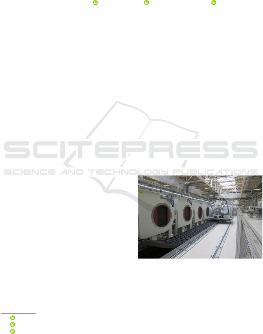
shown in Figure 1. There, parts of the future gear

shafts are hardened. The operating temperature of the

furnaces is 960

◦

C. Typically, the furnaces are heated

https://orcid.org/0000-0002-7365-844X

https://orcid.org/0000-0003-4895-157X

https://orcid.org/0000-0002-8135-1296

Figure 1: A steel hardening production line in

Skoda Auto

consisting of electrical vacuum furnaces (Du

sek, 2016).

to the operating temperature at the beginning of the

weak, and cooled down at its end. However, some

of the furnaces might not be utilized all the time, de-

pending on the previous production stages.

If the furnace is underutilized, energy can be saved

by lowering the temperature during the idle periods.

However, the furnace needs to be heated back to the

operating temperature before the next job arrives. As

Benedikt, O., Š˚ucha, P. and Hanzálek, Z.

On Idle Energy Consumption Minimization in Production: Industrial Example and Mathematical Model.

DOI: 10.5220/0008877400350046

In Proceedings of the 9th International Conference on Operations Research and Enterprise Systems (ICORES 2020), pages 35-46

ISBN: 978-989-758-396-4; ISSN: 2184-4372

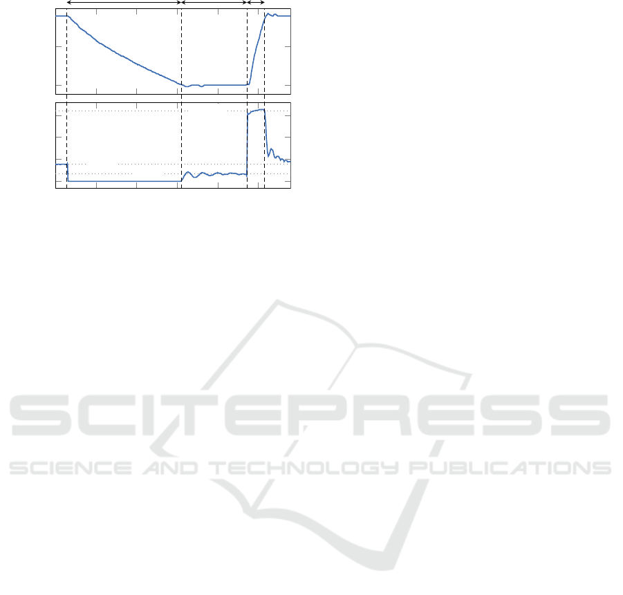
600

800

960

Temperature [

◦

100

150

200

250

100

150

160 kW

40 kW

18 kW

Time [min]

Power [kW]

cooling holding heating

Figure 2: A relationship between the power consumption

and the temperature of a single furnace during the experi-

ment.

re-heating of the furnace takes time and consumes en-

ergy, it needs to be planned carefully. Our prelim-

inary study in

Skoda Auto company has shown that

over 5 % of the energy consumption of the harden-

ing line could be saved by switching the idle furnaces

to the power-saving modes (Du

sek, 2016). Several

experiments were performed to investigate the poten-

tial for energy savings. During one of the experi-

ments, the furnace was heated to the operating tem-

perature, i.e., 960

◦

C; afterward, it cooled to 600

◦

and was re-heated back to 960

◦

C. Figure 2 shows

the relationship between the temperature and power.

Note that during the cooling phase, the input power is

zero. On the other hand, the maximal power (160 kW)

is applied for the re-heating to reach the operating

mode as soon as possible. The experiment shows

that the power needed to compensate for the losses

when holding 960

◦

C (about 40 kW) is more than two

times higher than the power needed for 600

◦

C (about

18 kW). That indicates the potential for energy sav-

ing. Of course, if the machine were turned off com-

pletely (i.e., to the ambient temperature), the power

consumption during the holding phase would be zero.

However, the complete cooling and re-heating would

require a considerably longer time (which might not

be available). Also, the energy needed for re-heating

would be higher. Therefore, depending on the idle

period length, different savings might be achieved by

cooling to different temperatures.

1.1 Contributions and Outline

This study aims to contribute to the growing area of

energy optimization research by providing an exam-

ple of the parallel machine problem, its formal de-

scription, and a formulation of a Mixed Integer Lin-

ear Programming (MILP) model. Compared to the

other problems of the idle energy optimization stud-

ied in the literature, this one is special because the

slow dynamics of the machine (furnace) and its “in-

ner state” (temperature) cannot be neglected. The

proposed MILP model takes into account possible

power-saving modes indirectly by using the energy

function, which abstracts the dynamics of the ma-

chine. The proposed model is compared with an-

other MILP model, adapted from the literature, and

its performance is further tested on a set of bench-

mark instances. Also, this paper shows that the en-

ergy function can easily replace conventional model-

ing approaches (e.g., those using on/off or on/idle/off

modes).

The rest of the paper is organized as follows. Sec-

tion 2 summarizes connections to relevant literature.

Section 3 formally describes the studied scheduling

problem. Afterward, the abstraction used for idle en-

ergy optimization, called the energy function, is in-

troduced in Section 4, together with several exam-

ples from the literature. Section 5 describes the MILP

model, which integrates the energy function. In Sec-

tion 6, the proposed model is compared to a reference

model, and its scalability is tested on a range of in-

stances. Finally, Section 7 gives a summary of the

ﬁndings.

2 RELATED WORK

In the area of production scheduling, one of the

ﬁrst analyses of underutilized machines was done by

Mouzon et al. (2007), who observed that changing

the machine modes could reduce energy consumption

signiﬁcantly. Furthermore, they proposed a mathe-

matical model to optimize energy and the completion

time by turning the machine on and off. However, the

model optimized a single machine only, assuming a

ﬁxed order of the jobs.

In the domain of single machine problems, Shrouf

et al. (2014) proposed a mathematical model and

heuristics for a single machine with three modes (pro-

cessing, idle and shut down), assuming variable en-

ergy prices. Gong et al. (2016) also addressed a prob-

lem with dynamic energy pricing, modeling a sin-

gle machine with multiple processing modes by a ﬁ-

nite state automaton. After completion of each job,

the machine could stay idle, shut down, or start pro-

cessing the next job. No power-saving modes be-

sides the shutdown mode were allowed. Furthermore,

it was assumed that transitions between the individ-

ual modes of the machine are immediate. This as-

ICORES 2020 - 9th International Conference on Operations Research and Enterprise Systems

sumption cannot be used here, because heating and

cooling take time. A single machine problem was

also investigated by Che et al. (2017), who optimized

weighted energy consumption and makespan and de-

ployed cluster analysis to approximate Pareto fronts

of large-size problems. Their problem statement is

similar to ours, but they scheduled on and off modes

only, which might be too restrictive when the com-

plete power-down takes a long time.

Compared to the single machine problem, paral-

lel machine scheduling studied here is much harder,

because the assignment of the jobs to machines needs

to be found together with their relative order and start

times. Fang and Lin (2013) described a MILP model,

dispatching heuristics, and a particle swarm optimiza-

tion algorithm for the weighted tardiness/cost prob-

lem. They assumed that the processing time of a job

could be shortened by increasing the speed of the ma-

chine, which is not the case for the problem studied

here because the hardening process needs to follow a

given technological speciﬁcation. Furthermore, their

MILP model was relatively slow even for ﬁve jobs

scheduled on three machines. Liang et al. (2015) for-

mulated a non-linear model of an on/off problem with

unrelated parallel machines and proposed an ant opti-

mization heuristic. Masmoudi et al. (2017) developed

a mathematical model and heuristic for a ﬂow shop

problem with time-of-use energy pricing, and Meng

et al. (2019) proposed MILP models for a ﬂexible job

shop problem, where on and off modes of the ma-

chines were considered. Benedikt et al. (2018) for-

mulated a parallel machine scheduling problem with

multiple processing modes with different processing

speeds and power consumption. A decomposition-

based approach based on the column generation tech-

nique was proposed to solve the problem. However,

the resulting mathematical models are still very com-

plex and have limited scalability. M

odos. et al.

(2019) studied a scheduling problem with dedicated

machines, inspired by glass tempering and steel hard-

ening processes. Instead of energy minimization, the

energy consumption limit (imposed for each metering

interval) was considered. However, the authors did

not model the power-saving modes of the machine,

which might have a positive impact on energy con-

sumption in the metering intervals when some of the

machines are idling.

Reviews of energy-efﬁcient scheduling were pub-

lished by Gahm et al. (2016) and Gao et al. (2019),

who summarized the latest trends in the area. The re-

views show that interest in energy-efﬁcient schedul-

ing is steadily increasing year by year. Also, the

reviews show that a mixed-integer (linear) program-

ming is one of the standard modeling techniques used

in the area.

We conclude that although the idle energy mini-

mization is widely studied, only two or several modes

of the machines are commonly modeled, which might

be too restrictive. Also, the unifying concept of the

idle energy consumption modeling (i.e., the energy

function) is still not widely known.

3 PROBLEM STATEMENT

3.1 Input Parameters and Assumptions

We consider a ﬁnite set of jobs J = {J

, J

, . . ., J

}

and a ﬁnite set of parallel identical machines M =

, M

, . . ., M

}. Each job J

is characterized by

three non-negative integers: processing time p

, re-

lease time r

, and deadline

. Release time and dead-

line form an execution time window within which the

job needs to be processed. Each job can be processed

on any machine, but each machine can process only

a single job at a time. When the processing starts, it

cannot be preempted.

While a job is processed, the machine needs to be

operating in a processing mode (heated to predeﬁned

operational temperature T

oper

) and cannot change it

until the processing of the job is ﬁnished. The pro-

cessing of job J

consumes energy E

(proc)

. When a

machine does not process any job, it enters a so-called

idle period. During the idle period, the temperature

can be changed to achieve energy savings, but when

the next job arrives, the machine needs to be heated

back to T

oper

. The relationship between energy con-

sumption and the length of the idle period ∆ is given

by energy function E : R

≥0

→ R

≥0

. For ﬁxed ∆, value

E(∆) represents the best attainable energy consump-

tion across all available machine modes. The energy

function is further discussed in Section 4.

It is assumed that each machine starts and ends

in “off-mode”, which has zero power consumption.

Some machines may remain in the off-mode all the

time, but at least one machine needs to be turned on

to process the jobs. The energy needed for the switch-

ing from off-mode to the processing mode and back

is given by E

(start)

∈ R

. It is assumed that there

is enough time to turn the machines on before the

ﬁrst job is available and to turn them off after the last

job is processed. In the following text, the length

of the scheduling horizon is denoted by H, where

H = max{

| J

∈ J }.

On Idle Energy Consumption Minimization in Production: Industrial Example and Mathematical Model

3.2 Solution Representation

Solution S can be represented by a pair of vec-

tors, S = (a

a, s

s), where vector s

s = (s

, . . ., s

) ∈ Z

≥0

represents start times of the jobs, and vector

a = (a

, . . ., a

) ∈ M

captures assignment of the

jobs to machines. The solution is feasible if all jobs

are processed within their execution windows without

preemption or overlapping.

3.3 Optimization Objective

The assignment of the jobs, together with their start

times, deﬁne the idle periods in the schedule. De-

pending on their lengths, energy consumption may

vary.

Before deﬁning the objective, let us denote the in-

dex of the job scheduled immediately before job J

solution S on machine a

by pred

(i). If such a job

does not exist, i.e., the job J

is the ﬁrst on machine

, we deﬁne pred

(i) := 0. Now, the energy con-

sumption corresponding to solution S can be written

as follows:

∑

i=1

(proc)

∑

i=1

pred

(i)6=0

E(s

− s

pred

(i)

− p

pred

(i)

) +

∑

i=1

pred

(i)=0

(start)

(1)

where the ﬁrst sum represents the total energy needed

to process the jobs, the second sum corresponds to

the energy consumed during the idle periods (energy

function E is further described in Section 4), and the

third sum express the energy needed for turning the

machines (to which at least one job is assigned) on

and off. The optimal schedule minimizes the total en-

ergy consumption (1).

Note that constant

∑

i=1

(proc)

can be omitted for

the optimization as it does not affect the structure of

the optimal schedule.

3.4 Complexity

Using the standard α|β|γ notation, we can character-

ize the studied problem as P|r

idle

, meaning idle

energy minimization for parallel identical machines

and jobs characterized by release times and dead-

lines. The problem is N P -hard because its subprob-

lem 1|r

|− is already N P -complete in the strong

sense (Garey and Johnson, 1977).

4 ENERGY FUNCTION

The energy function is a concept used when idle en-

ergy minimization is taken into account. The spe-

ciﬁc properties of the resource are abstracted, and

only the information about the energy consumption

is explicitly represented. This concept often simpli-

ﬁes the analysis of the problem properties, as well as

the models and algorithms. Here, we establish the

basic notions in Section 4.1 and show several exam-

ples from the literature in Section 4.2. Afterward, we

discuss the energy function obtained for vacuum fur-

naces studied in this paper in Section 4.3.

4.1 Basic Notions

Denoting V the set of all machine modes, a basic ma-

chine model can be described as follows. When the

machine processes a job, it needs to be operating in

the processing mode “proc”. When no job is pro-

cessed, the machine can change the mode. Switch-

ing to (non-processing) mode v and back takes time

, and consumes energy E

. The power consump-

tion of the machine in mode v is denoted by P

, and is

assumed to be constant. Depending on the length of

the idle period between two neighboring jobs, which

is denoted by ∆, a machine can either turn to some

non-processing mode (and back) or remain in the pro-

cessing mode. Clearly, if ∆ is shorter than T

, switch-

ing to mode v is not feasible. Also, switching to a

power-saving mode should be only performed when

it would not increase the overall power consumption

(Devadas and Aydin, 2012). These observations lead

us to the following formulation of the energy con-

sumption function E : R

≥0

→ R

≥0

(Gerards and Ku-

per, 2013):

E(∆) = min

v∈V :∆≥T

+ P

· (∆ −T

)}. (2)

Formally, we deﬁne T

proc

= E

proc

= 0, i.e., for

V = {proc}, E(∆) = P

proc

· ∆.

The value E(∆) represents the best attainable en-

ergy consumption for given idle period length ∆. Note

that the optimal mode to which the machine should be

switched is given by the argument of the minimum in

(2). In the following section, we discuss several ap-

plications of this model.

4.2 Examples from the Literature

Concept of the idle energy minimization is relatively

old. Initially, the possibilities of the power savings

were investigated in the ﬁeld of embedded systems

(Benini et al., 2000; Augustine et al., 2008; Gerards

ICORES 2020 - 9th International Conference on Operations Research and Enterprise Systems

0 20 40

·10

processing

mode 1

mode 2

mode 3

mode 4

∆ [ms]

E [mJ]

processing

mode 1

mode 2

mode 3

mode 4

Figure 3: The energy function of a sensor node from em-

bedded systems domain (Sinha and Chandrakasan, 2001).

and Kuper, 2013), where energy consumption plays

a critical role for the lifetime of the battery-powered

systems. Nowadays, it is common that hardware com-

ponents have one or several power-saving modes de-

ﬁned by the manufacturer (Gerards and Kuper, 2013).

Of course, the time and energy needed to perform the

transitions between the modes are usually not negligi-

ble. Therefore, the selection of the “optimal” power-

saving mode of the component depends on the idle

period length.

An example of a hardware device with multiple

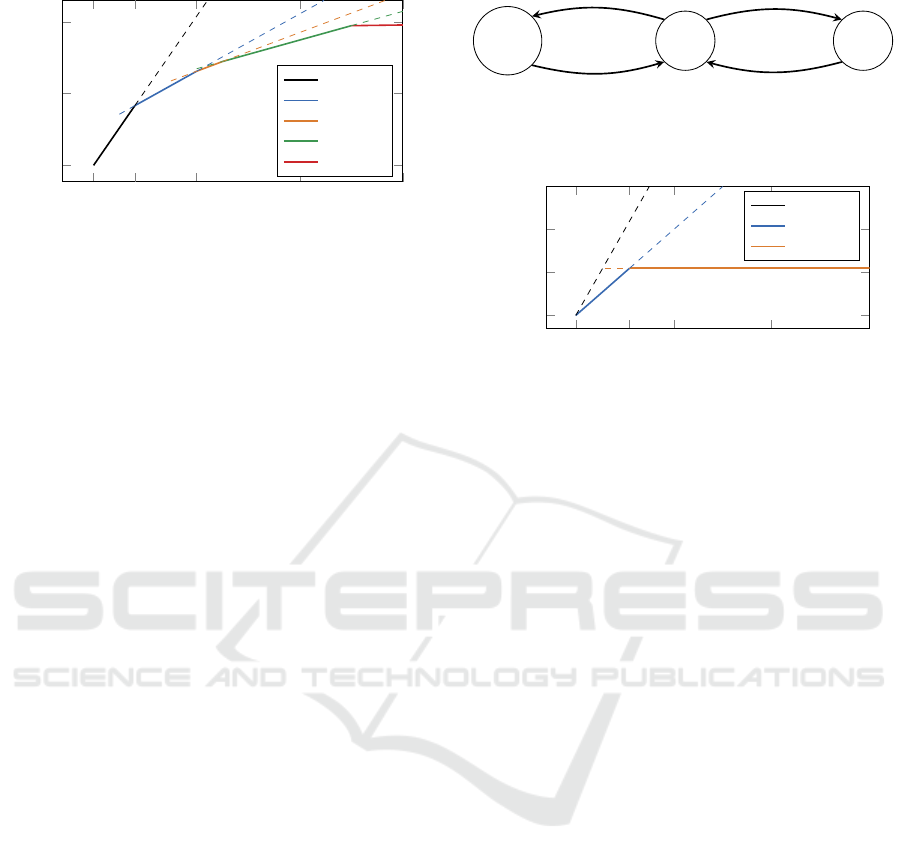
modes is a sensor node (Sinha and Chandrakasan,

2001), which has four power-saving modes, with T

equal to 5, 15, 20, and 50 milliseconds, respectively.

The piecewise linear function drawn by a solid line in

Figure 3 is the energy function of the device. It con-

sists of 5 segments, corresponding to different modes

of the device. Note that even though mode 1 is acces-

sible already for ∆ = 5, it is not proﬁtable to perform

the switching until ∆ = 8, which is called a break-even

time in the literature (Devadas and Aydin, 2012).

In the production domain, research of the idle en-

ergy minimization is still relatively new. The interest

in the topic increased after Mouzon’s study, which an-

alyzed underutilized machines (Mouzon et al., 2007).

Since that time, researchers have started to take the

power-saving modes of the machines into consider-

ation. However, only a small number of modes is

usually considered (Shrouf et al., 2014; Che et al.,

2017; Aghelinejad et al., 2019). Typically, the ma-

chine modes and transitions are modeled by a transi-

tion graph. A representative example of such a graph

is shown in Figure 4 (Shrouf et al., 2014). The nodes

are labeled by power consumption, while the edges

are labeled by energy/time needed for the transition.

Parameters needed for the energy function can be eas-

ily obtained from the graph. For example, T

off

= 3 h,

off

= 11kW h, P

off

= 0kW, etc. The corresponding

energy function is shown in Figure 5.

standby

proc

off

2 kW 4 kW

0 kW

0 kW h / 0 h

10 kW h / 2 h

1 kW h / 1 h

Figure 4: Example of a transition graph depicting machine

modes and transitions between them (Shrouf et al., 2014).

0 10 20 30

5.5

processing

standby

off

∆ [h]

E [kW h]

processing

standby

off

Figure 5: Energy function corresponding to the transition

graph depicted in Figure 4.

4.3 Energy Function and Industrial

Furnaces

When considering the industrial furnaces, the situ-

ation is slightly more complicated because of their

slow dynamics. Depending on the input power, the

furnace is either cooling (temperature inside is de-

creasing), holding (temperature inside is stable), or

heating (temperature inside is increasing), as shown

in Figure 2. We could associate the mode v of the

furnace with the temperature that should be held in-

side of the furnace. The power consumption P

is then

the power needed to compensate for the steady-state

losses of the furnace. The switching time T

is the

time needed for cooling plus the time needed for re-

heating, and the switching energy consumption E

equal to the energy needed for cooling (which equals

zero) and the energy needed for re-heating.

Now, if we wanted to model such a system by a

transition graph, we would face a problem, as only a

ﬁnite number of machine modes can be modeled like

that. On the other hand, the temperature in the fur-

nace can be changed continuously, and so an inﬁnitely

large set V would be needed to model all possible

power-saving modes.

Figure 6 shows two possible energy functions of

the furnace corresponding to two different control

strategies. Function E

600

represents a standard ap-

proach using a transition graph with a single power-

saving mode associated with the temperature 600

◦

The corresponding control rule states: cool to 600

◦

hold 600

◦

C as long as possible and re-heat to the

operating temperature as fast as possible just be-

fore the end of the idle period. The slope of the

On Idle Energy Consumption Minimization in Production: Industrial Example and Mathematical Model

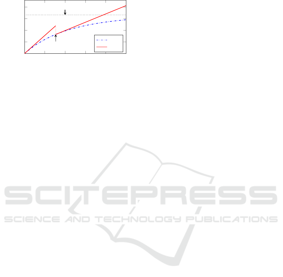
0 100 200 300 400

500

120

160

asymptote of E

cont

600

processing

holding 600

◦

∆ [min]

E [kW h]

cont

600

Figure 6: Energy function of an industrial furnace E

cont

in-

tegrating all power-saving modes (Benedikt et al., 2019),

and function E

600

corresponding to a single power-saving

mode.

ﬁrst segment of E

600

corresponds to the power con-

sumption of the processing mode, while the slope of

the second segment corresponds to the power com-

pensating for the losses when holding 600

◦

C. Energy

600

) is the energy needed to re-heat the furnace

from 600

◦

C back to the 960

◦

C (remember that en-

ergy needed for cooling is zero). Transition to the

power-saving mode is not possible during time inter-

val [0, T

600

), because there is not enough time to cool

the furnace to 600

◦

C and re-heat it back.

On the other hand, function E

cont

is a result

of a detailed analysis of the industrial furnace, see

Benedikt et al. (2019). The control rule states that

the furnace should be cooling as long as possible, and

should be re-heated as fast as possible to reach the

operating mode again at the end of the idle period.

With the increasing length of the idle period, the tem-

perature to which the furnace cools decreases until it

reaches the ambient temperature. Then, the energy

needed to cool to the ambient temperature and to re-

heat back corresponds to the asymptote shown by the

dashed line.

Note that when only a subset of all modes is con-

sidered, the energy function becomes discontinuous,

like E

600

. The reason for the discontinuity is that the

cooling of the furnace is slow, and so the integral of

the processing power over interval [0, T

600

] becomes

greater than the switching energy consumption E

600

Contrary to that, function E

cont

, which implicitly rep-

resents all possible temperatures, remains continuous

and concave (similarly to the energy functions shown

in Figures 3 and 5).

5 MATHEMATICAL MODEL

In this section, we integrate the energy function into

a MILP model proposed for the problem deﬁned in

Section 3.

As shown by Gahm et al. (2016), formulating

problems by MILP models and solving them by

standard solvers has been one of the widely used

approaches to the optimal energy-aware schedul-

ing. There exist several alternative approaches to the

scheduling problem modeling in MILP. Many authors

use time-indexed models (Shrouf et al., 2014; Mitra

et al., 2012; Masmoudi et al., 2017) – scheduling hori-

zon is divided into periods and decisions about the

mode of the machine or assignment of jobs have to

be made for each period separately. In many cases,

the time-indexed models are the only reasonable al-

ternative, e.g., when the properties of the system vary

through time. However, the size of a time-indexed

model depends on the length of the scheduling hori-

zon, which is prohibitive.

Other formulation approaches use event-based

modeling (Kon

e et al., 2011), permutation (position-

based) models (Che et al., 2017), or relative order

models (Liang et al., 2015).

The model we propose in this work is a special

variant of the relative-order model, modeling the di-

rect predecessor and successor of each job. A similar

idea has already been used in the scheduling domain

successfully (Liu et al., 2008). However, we inte-

grate the concept of the energy consumption function

into the model formulation to describe the transition

costs efﬁciently. The model is compared to a position-

based model in Section 6.

5.1 Model Description

At ﬁrst, we deﬁne two dummy jobs; the ﬁrst one,

(dummy-start), is ﬁxed to start and end at time

0, while the second one, J

(dummy-end), must start

and end at time H. Both have zero processing length.

These dummy jobs model the predecessor (successor)

of the ﬁrst (last) job assigned to each machine.

5.1.1 Variables

We use ﬁve types of variables to model the problem.

Binary variables are:

i,k

indicates if job J

is assigned to machine M

i, j,k

decides whether job J

immediately precedes

job J

on machine M

indicates whether at least one job is assigned

to machine M

Continuous variables follow:

corresponds to start time of job J

i, j

equals to the length of the idle period between

jobs J

and J

if J

immediately precedes J

otherwise 0

ICORES 2020 - 9th International Conference on Operations Research and Enterprise Systems

Variables y

i, j,k

are deﬁned for jobs including the

dummies. All the other variables are deﬁned for non-

dummy jobs only. Note that variables z

i, j

model the

lengths of idle periods ∆.

5.1.2 Objective

As discussed in Section 3.3, the objective is to min-

imize the total idle energy consumption plus the en-

ergy needed to power the machines up and turn them

down (if there is at least one job assigned to the ma-

chine). Using the deﬁned variables, we can write the

whole objective as

∑

i∈J

∑

j∈J

i6= j

E(z

i, j

) + E

(start)

∑

k∈M

. (3)

The non-linear energy function E is approximated

by a piecewise linear function. The approximation

can be made simply and with high precision even

with a small number of segments, thanks to the simple

shape of the energy function.

Note that functions corresponding to ﬁnite transi-

tions graph, such as the ones shown in Figure 3 and

Figure 5, are already piecewise linear by deﬁnition

(2).

The piecewise linear objective function can be fur-

ther linearized by introducing additional binary and

continuous variables. However, modern solvers, such

as Gurobi or CPLEX, can optimize piecewise linear

objectives natively. The linearization is handled inter-

nally, and solvers may even beneﬁt by using special-

ized data structures and algorithms.

5.1.3 Constraints

Equations (4) force each job to be assigned to exactly

one machine. Constraints (5) and (6) deﬁne that if job

is scheduled to machine M

, it has exactly one im-

mediate predecessor and successor on that machine,

and otherwise if it is not assigned to machine M

it cannot precede and follow any other job on that

machine. Constraints (7) and (8) force dummy-start

(dummy-end) to have exactly one successor (prede-

cessor) on each machine. Execution time windows

of the jobs are established by (9), whereas constraints

(10) forbid overlapping of the neighboring jobs. In-

equalities (11), (12) and (13) link variable z

i, j

to the

length of the respective idle period. If job J

pre-

cedes job J

on some machine, z

i, j

is exactly equal

to s

− (s

+ p

), i.e., to the length of the idle period

between those two consecutive jobs; otherwise, it is

set to zero. Finally (14) forces x

to 1, if there is at

least one job assigned to this machine. Symbol M

represents some large constant (e.g., M = H).

∑

∈M

i,k

= 1, J

∈ J (4)

∑

∈J ∪{J

}

j6=i

i, j,k

= a

i,k

, J

∈ J , M

∈ M (5)

∑

∈J ∪{J

}

j6=i

j,i,k

= a

i,k

, J

∈ J , M

∈ M (6)

∑

∈J ∪{J

}

j,i,k

= 1, M

∈ M , J

= J

(7)

∑

∈J ∪{J

}

i, j,k

= 1, M

∈ M , J

= J

(8)

≤ s

≤

− p

, J

∈ J (9)

+ p

+ z

i, j

≤ s

+ M ·(1 − y

i, j,k

∈ J , J

∈ J , M

∈ M

(10)

− (s

+ p

) ≤ z

i, j

+ M ·(1 −

∑

∈M

i, j,k

∈ J , J

∈ J , i 6= j

(11)

− (s

+ p

) ≥ z

i, j

− M ·(1 −

∑

∈M

i, j,k

∈ J , J

∈ J , i 6= j

(12)

i, j

≤ M ·

∑

∈M

i, j,k

, J

∈ J , J

∈ J , i 6= j (13)

≥ (1 − y

i, j,k

), M

∈ M , J

= J

, J

= J

(14)

Besides the constraints mentioned above, which

deﬁne the behavior of the model, additional con-

straints can be added to reduce the search space by

eliminating symmetries. Constraints (15) state that

jobs are preferably assigned to machines with lower

indices. Constraints (16) pre-assign the ﬁrst job to the

ﬁrst machine, the second job to the ﬁrst or the second

machine, etc.

≥ x

k+1

, M

∈ {1, . . . , m − 1} (15)

∑

k=1

i,k

= 1, i ∈ {1, . .. , min{m, n}} (16)

To further reduce the solution space, we use ad-

ditional constraints that link the lengths of the gaps

with the start times of the jobs – stating that all the

gaps and jobs should ‘ﬁll’ the whole scheduling hori-

zon. For that, we add new variables start

and end

which denote the start time of the ﬁrst job processed

on machine M

, and the ending time of the last job

processed on machine M

, respectively. It must hold

that if job J

follows immediately after J

on ma-

chine M

, then start

= s

. Similarly, if job J

im-

mediately precedes J

on machine M

, then end

H − (s

+ p

), where H is the length of the schedul-

ing horizon. These logical implications in the form

On Idle Energy Consumption Minimization in Production: Industrial Example and Mathematical Model

if x = 1 then y = z with binary variable x and continu-

ous variables y and z can be linearized by introducing

two constraints:

y − z ≤ M(1 − x), and z − y ≤ M(1 − x).

Now, constraint (17) can be added:

∑

i=1

∑

i=1

∑

j=1

i6= j

i, j

∑

k=1

(start

+ end

) = H

∑

k=1

(17)

6 EXPERIMENTS

To test the performance of the proposed model, we

conduct two types of experiments. The ﬁrst experi-

ment compares our model to the position-based model

adopted from the relevant paper (Che et al., 2017),

and the second experiment examines the scalability

of our model on larger problem instances.

For each experiment, a wide range of instances is

generated for different combinations of n and m. The

optimality gap is used to measure the performance of

the model(s). In the following text, U{x, y} stands

for an integer uniform distribution on interval [x, y],

Exp(x) denotes the exponential distribution with scale

parameter x, and E(p

) represents the expected pro-

cessing time of job i.

All experiments were performed on a Dell PC

with an Intel Core i7-4610M CPU operating at 3 GHz,

16 GB RAM. Gurobi Optimizer (version 8.1) was

used to solve the MILP models.

6.1 Benchmark Data

Jobs’ parameters are generated according to the fol-

lowing scheme. At ﬁrst, vector a

a = (a

, . . ., a

) is

generated, a

∼ U{1, m}, describing the random as-

signment of the jobs to machines. Note that vector

a is used only for data generation, simulating the pro-

duction process. It might be different from the assign-

ment found by the optimization solver.

Processing times, release times, and deadlines are

generated according to (18), (19) and (20), respec-

tively.

∼ U{p

min

, p

max

} (18)

∼

i−1

∑

k=1

= a

K · E(p

) + Exp(α· E(p

)) (19)

∼ r

+ p

+ β ·E(p

) + Exp(γ· E(p

)) (20)

Processing times, release times, and deadlines are

assumed to be integers, so only the upper integer part

of the generated data is considered. Symbols p

min

max

, α, β and γ represent parameters, which allow us

to generate instances with different properties. Indi-

cator Ja

= a

K is one if a

= a

, and zero otherwise.

Experiment 1: Comparison with a Position-based

Model

In this experiment, we compare our model to the

position-based model, which was originally devel-

oped by Che et al. (2017) for a single machine prob-

lem. As the problem studied in this paper differs from

the problem studied by Che et al., it was necessary to

modify their model slightly. The modiﬁed model is

described in Appendix. For both models, additional

constraints (15–17), and (29–31) were used.

Because the reference position-based model opti-

mizes the energy consumption for two modes only,

energy function E

600

with a single switching depicted

in Figure 6 was used for the experiment. There

were 50 testing instances randomly generated for each

combination of n ∈ {10, 15, 20}, m ∈ {1, 2, 4}, α ∈

{0.8, 1.2} and γ ∈ {1, 1.5}; (1800 instances in total).

Parameter β was set to 1. The minimal and maximal

processing times p

min

, and p

max

, were set to 1 and

300, respectively. The time limit was set to 300 s per

instance.

The overall results of the experiment are shown in

Table 1. Each row aggregates 200 instances; 50 gen-

erated for each combination of α and γ. A number

of infeasible instances is given by #if. A number of

timeouts is listed in the table in the columns #to. The

average runtimes are measured and listed for feasi-

ble and infeasible instances separately, where t

and

represent the average time over infeasible and fea-

sible instances, respectively. Average times that are

typed in the bold font mark the better of the two tested

solvers. The average optimality gap is listed as well

(computed over all instances aggregated in the given

row). Solving times aggregated over all feasible in-

stances are also depicted in Figure 7 in the form of

box plots.

The single machines instances were solved by

both models without any problems. The performance

of the position-based model was slightly better. How-

ever, the absolute times of both models were low. In-

stances with parallel machines are harder to solve be-

cause the assignment needs to be found together with

the order of the jobs. Results show that our model

outperformed the reference model when the number

of machines was higher than 1. The biggest differ-

ence can be seen for m = 2, n = 20, where the refer-

ence model ran out of time three times more often,

ICORES 2020 - 9th International Conference on Operations Research and Enterprise Systems

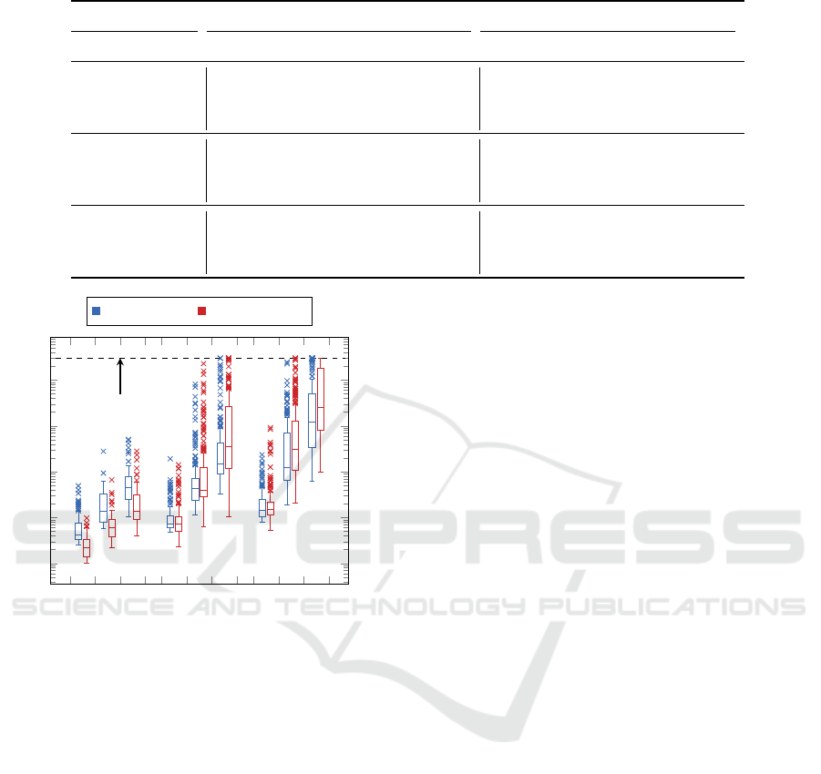
Table 1: Comparison between the position-based model and the relative-order model.

Instances Position-based (reference) Relative-order (this work)

n m #if #to t

[s] t

[s] gap [%] #to t

[s] t

[s] gap [%]

1 87 0 0.01 0.03 0.00 0 0.03 0.08 0.00

10 2 6 0 0.39 0.12 0.00 0 0.41 0.12 0.00

4 0 0 - 0.37 0.00 0 - 0.24 0.00

1 126 0 0.02 0.08 0.00 0 0.07 0.24 0.00

15 2 12 1 56.09 6.29 0.00 0 1.99 2.38 0.00

4 0 4 - 23.80 0.45 0 - 8.64 0.00

1 148 0 0.04 0.35 0.00 0 0.19 0.88 0.00

20 2 23 29 190.60 43.09 1.65 9 95.92 16.79 0.23

4 0 41 - 96.12 6.73 23 - 61.66 3.48

10-1 15-1 20-1 10-2 15-2 20-2 10-4 15-4 20-4

−2

−1

time limit

Parameters n-m

Time [s]

Relative-order Position-based

Figure 7: Comparison between the relative-order model

(left) and the position-based model (right) of the solving

times on feasible instances for different pairs of n and m.

and performed more than 2.5 times slower on the fea-

sible instances on average. The difference is not that

large for m = 4, n = 20, because both models started

to reach the maximum solving time (see Figure 7).

Considering the optimality gap, the average over-

all instances for which at least one of the models did

not ﬁnd an optimal solution was 23.02 % for the ref-

erence model and 9.84 % for our model.

The total run time was 37 987 s for the reference

model and 19 894 s for our model, so our model was

nearly two times faster on average. Furthermore, it is

important to note that our model can optimize any en-

ergy function, which can be approximated by a piece-

wise linear function, whereas the reference model was

developed to optimize the on/off modes only.

Experiment 2: Scalability

In the second experiment, the proposed model is

tested on larger instances. For the experiment, a

piecewise linear approximation of energy function

cont

shown in Figure 5 was used. The approxi-

mation was made by 17 linear segments. Ten in-

stances were generated for each combination of n ∈

{20, 25, 30, 35}, m ∈ {2, 4,6}, α ∈ {1, 1.5}, and γ ∈

{1, 2}; 480 instances in total. Parameter β was set to

1. Parameters p

min

and p

max

were again set to 1 and

300, respectively. The maximal time limit was set to

10 min per instance.

The results are listed in Table 2. Each row aggre-

gates 40 instances generated for each combination of

α and γ. Column #if shows the number of infeasible

instances, #to

(#to

) represents the number of time-

outs on infeasible (feasible) instances, t

) is the

average time on the respective instances, and ‘gap’ is

the average optimality gap over the feasible instances,

for which some solution was found.

Table 2 shows how the complexity increases with

the increasing number of jobs and machines. The

performance of the model, which includes additional

constraints (15), (16), and (17), is compared to the

same model without these constraints.

The results show that the additional constraints

signiﬁcantly improve the behavior of the model.

The overall average optimality gap decreases from

40.73 % to 14.20 % when the constraints are used.

Also, the number of optimally solved instances in-

creases from 119 to 233, and the number of timeouts

decreases from 343 to 226. The ability to ﬁnd a fea-

sible solution is comparable for both models – model

without symmetry breaking constraints ﬁnds a solu-

tion to 414 instances, while the model with symmetry

breaking constraints ﬁnds a solution to 433 instances

(out of 450 feasible instances).

On Idle Energy Consumption Minimization in Production: Industrial Example and Mathematical Model

Table 2: Performance of the relative-order model on larger instances.

Instances Relative-order (without additional constr.) Relative-order (with additional constr.)

n m #if #to

#to

[s] t

[s] gap [%] #to

#to

[s] t

[s] gap [%]

2 10 1 3 94 103 4.39 0 2 56 56 0.41

20 4 0 0 26 - 452 36.07 0 11 - 220 7.98

6 0 0 30 - 501 47.17 0 13 - 235 11.26

2 4 2 10 305 229 7.22 1 5 157 141 2.27

25 4 0 0 33 - 531 50.50 0 15 - 270 12.08

6 0 0 39 - 593 62.24 0 25 - 432 19.18

2 8 7 12 526 334 16.10 7 9 527 220 5.15

30 4 0 0 38 - 574 55.89 0 27 - 464 23.44

6 0 0 40 - 600 63.95 0 32 - 518 25.99

2 8 6 17 465 367 16.78 4 13 363 337 5.77

35 4 0 0 39 - 592 54.65 0 24 - 481 18.40

6 0 0 40 - 600 65.95 0 38 - 581 32.38

When the instances are large, it may be hard to

ﬁnd a feasible solution or detect the infeasibility.

However, this could be solved by a simple decompo-

sition, using, for example, some heuristics or a Con-

straint programming model to check feasibility and

possibly provide a feasible assignment as an initial

solution to the MILP model.

7 CONCLUSIONS

This study addresses the modeling of an idle energy

minimization scheduling problems. The technique of

implicit modeling of the machine modes called idle

energy function, which abstracts dynamics of the ma-

chine and provides a link between the idle period

length and the optimal idle energy consumption, is

adopted from the domain of embedded systems. It is

shown that this method is applicable to a wide range

of idle energy minimization problems. Furthermore,

discussed examples illustrate that the properties of the

problems are similar across different domains, and the

shape of the energy function is the same for many rel-

evant applications.

An efﬁcient MILP model that uses the idle energy

function is proposed to solve the scheduling problem

optimally. The proposed model is compared to the

position-based model adapted from the literature. The

experiment shows that the overall performance of our

model is signiﬁcantly better when the number of ma-

chines was higher than one, even though the refer-

ence model is less general. Besides the comparison,

another experiment is conducted to show the perfor-

mance of the proposed model and the effect of the

symmetry breaking constraints on larger instances of

the problem. The importance of the additional con-

straints is apparent, as the overall optimality gap de-

creases nearly three times when the constraints are

used.

In our future research, we would like to inte-

grate the idle energy function into heuristics to solve

industrial-size instances of the problem. Also, we

want to investigate multi-objective optimization, be-

cause the trade-off between energy consumption and

productivity-related objectives (such as makespan or

the total tardiness) is known and widely studied.

ACKNOWLEDGEMENTS

This work was funded by the Ministry of Ed-

ucation, Youth and Sport of the Czech Re-

public within the project Cluster 4.0 number

CZ.02.1.01/0.0/0.0/16 026/0008432. This work

was also supported by the Grant Agency of the

Czech Technical University in Prague, grant No.

SGS19/175/OHK3/3T/13.

REFERENCES

Aghelinejad, M., Ouazene, Y., and Yalaoui, A. (2019).

Complexity analysis of energy-efﬁcient single ma-

chine scheduling problems. Operations Research Per-

spectives, 6:100105.

Augustine, J., Irani, S., and Swamy, C. (2008). Op-

timal power-down strategies. SIAM J. Comput.,

37(5):1499–1516.

Benedikt, O., Alikoc¸, B.,

ucha, P.,

Celikovsk

y, S.,

and Hanz

alek, Z. (2019). A scheduling and con-

ICORES 2020 - 9th International Conference on Operations Research and Enterprise Systems

trol approach for an industrial furnace to mini-

mize idle energy consumption. arXiv e-prints, page

arXiv:1910.07501.

Benedikt, O.,

ucha, P., M

odos, I., Vlk, M., and Hanz

alek,

Z. (2018). Energy-aware production scheduling with

power-saving modes. In van Hoeve, W.-J., editor, Inte-

gration of Constraint Programming, Artiﬁcial Intelli-

gence, and Operations Research, pages 72–81, Cham.

Springer International Publishing.

Benini, L., Bogliolo, A., and Micheli, G. D. (2000). A

survey of design techniques for system-level dynamic

power management. IEEE Transactions on Very Large

Scale Integration (VLSI) Systems, 8(3):299–316.

Che, A., Wu, X., Peng, J., and Yan, P. (2017). Energy-

efﬁcient bi-objective single-machine scheduling with

power-down mechanism. Computers & Operations

Research, 85:172 – 183.

Devadas, V. and Aydin, H. (2012). On the interplay of

voltage/frequency scaling and device power manage-

ment for frame-based real-time embedded applica-

tions. IEEE Trans. Comput., 61(1):31–44.

sek, J. (2016). N

avrh

upravy

ızen

ı v

yrobn

ı linky s ohle-

dem na sn

zen

ı jej

ı spot

reby. Master’s thesis, Czech

Technical University in Prague, the Czech republic.

Fang, K.-T. and Lin, B. M. (2013). Parallel-machine

scheduling to minimize tardiness penalty and power

cost. Computers & Industrial Engineering, 64(1):224

– 234.

Gahm, C., Denz, F., Dirr, M., and Tuma, A. (2016). Energy-

efﬁcient scheduling in manufacturing companies: A

review and research framework. European Journal of

Operational Research, 248(3):744 – 757.

Gao, K., Huang, Y., Sadollah, A., and Wang, L. (2019).

A review of energy-efﬁcient scheduling in intelligent

production systems. Complex & Intelligent Systems.

Garey, M. and Johnson, D. (1977). Two-processor schedul-

ing with start-times and deadlines. SIAM Journal on

Computing, 6(3):416–426.

Gerards, M. E. T. and Kuper, J. (2013). Optimal DPM and

DVFS for frame-based real-time systems. ACM Trans.

Archit. Code Optim., 9(4):41:1–41:23.

Gong, X., Pessemier, T. D., Joseph, W., and Martens, L.

(2016). A generic method for energy-efﬁcient and

energy-cost-effective production at the unit process

level. Journal of Cleaner Production, 113:508 – 522.

Kon

e, O., Artigues, C., Lopez, P., and Mongeau, M. (2011).

Event-based MILP models for resource-constrained

project scheduling problems. Computers & Opera-

tions Research, 38(1):3 – 13. Project Management and

Scheduling.

Liang, P., dong Yang, H., sheng Liu, G., and hua Guo,

J. (2015). An ant optimization model for unrelated

parallel machine scheduling with energy consumption

and total tardiness. Mathematical Problems in Engi-

neering.

Liu, S., Pinto, J. M., and Papageorgiou, L. G.

(2008). A TSP-based MILP model for medium-

term planning of single-stage continuous multiproduct

plants. Industrial & Engineering Chemistry Research,

47(20):7733–7743.

Masmoudi, O., Yalaoui, A., Ouazene, Y., and Chehade,

H. (2017). Solving a capacitated ﬂow-shop prob-

lem with minimizing total energy costs. The Interna-

tional Journal of Advanced Manufacturing Technol-

ogy, 90(9):2655–2667.

odos., I., Kalodkin., K.,

ucha., P., and Hanz

alek., Z.

(2019). Scheduling on dedicated machines with en-

ergy consumption limit. In Proceedings of the 8th In-

ternational Conference on Operations Research and

Enterprise Systems - Volume 1: ICORES,, pages 53–

62. INSTICC, SciTePress.

Meng, L., Zhang, C., Shao, X., and Ren, Y. (2019). Milp

models for energy-aware ﬂexible job shop scheduling

problem. Journal of Cleaner Production, 210:710 –

723.

Mitra, S., Grossmann, I. E., Pinto, J. M., and Arora,

N. (2012). Optimal production planning under

time-sensitive electricity prices for continuous power-

intensive processes. Computers & Chemical Engi-

neering, 38:171 – 184.

Mouzon, G., Yildirim, M., and Twomey, J. (2007). Opera-

tional methods for minimization of energy consump-

tion of manufacturing equipment. International Jour-

nal of Production Research, 45:4247–4271.

Shrouf, F., Ordieres-Mer

e, J., Garc

ıa-S

anchez, A., and

Ortega-Mier, M. (2014). Optimizing the production

scheduling of a single machine to minimize total en-

ergy consumption costs. Journal of Cleaner Produc-

tion, 67:197 – 207.

Sinha, A. and Chandrakasan, A. (2001). Dynamic power

management in wireless sensor networks. IEEE De-

sign Test of Computers, 18(2):62–74.

APPENDIX

Here, the position-based MILP model used for the

comparison is described. It was originally proposed in

(Che et al., 2017) to minimize the total tardiness and

idle energy on a single machine with a single power-

saving mode.

Reference Model

The idea of the model is to represent all possible

positions to which the individual jobs can be as-

signed. The variable representing the completion time

is linked with the position instead of the job. A set

of constraints assure that if a job is assigned to some

position, its completion time is bounded (by the dead-

line, neighboring jobs, etc.). Following decision vari-

ables are used:

i,l,k

Binary variable; if job J

is assigned to position

l on machine M

. then x

i,l,k

= 1, otherwise 0

l,k

Binary variable; if there is turn-off-on opera-

tion immediately after l-th job is processed on

machine M

, then y

l,k

= 1, otherwise 0

On Idle Energy Consumption Minimization in Production: Industrial Example and Mathematical Model

l,k

Integer variable; completion time of l-th job on

machine M

l,k

Continuous variable; energy consumed by ma-

chine M

between the completion time of k-th

job and start of (k + 1)-th job

To simplify the notation, we substitute p

i,l,k

for

∑

i=1

i,l,k

· p

. Also, we substitute L for {1, 2, . . . ,n}.

In the following model, T

denotes the switching

time (i.e., the break-even time between the operating

and standby modes), and C

stands for the switching

cost; P

and P

represent the power consumed in the

processing mode and the standby mode, respectively.

Now, the whole model can be written as follows:

min

∑

k=1

n−1

∑

l=1

l,k

(21)

subject to

∑

l=1

∑

k=1

i,l,k

= 1, J

∈ J (22)

∑

i=1

i,l,k

≤ 1, l ∈ L, M

∈ M (23)

l,k

− p

i,l,k

≥

∑

i=1

i,l,k

· r

, l ∈ L, M

∈ M (24)

l,k

≤

∑

i=1



i,l,k



+ M ·

1 −

∑

i=1

i,l,k

l ∈ L, M

∈ M

(25)

l,k

≤ c

l−1,k

+ p

i,l,k

+ y

l,k

· T

, l ∈ L, M

∈ M

(26)

l,k

≥ (c

l+1,k

− c

l,k

− p

i,l,k

) · P

− M ·y

l,k

l ∈ L, M

∈ M

(27)

l,k

≥ C

· y

l,k

+ (c

l+1,m

− c

l,m

− p

i,l,k

− T

) · P

l ∈ L, M

∈ M

(28)

To improve the performance of the model, we add

several symmetry-breaking constraints. Constraints

(29) and (30) are analogous to constraints (15) and

(16), respectively. Constraint (17) cannot be easily

integrated into the described position-based model as

it does not use the variables z

i, j

. Instead, constraints

(31) are added, which enforce assignment order from

the leftmost position to the right.

∑

i=1

i,1,k

≥

∑

i=1

i,1,k+1

, k ∈ {1, . . . , m − 1} (29)

∑

l=1

∑

k=1

i,l,k

= 1, i ∈ {1, . .. , min{m, n}} (30)

∑

i=1

i,l,k

≥ x

i,l+1,k

, k ∈ {1, . . . , n − 1}, M

∈ M

(31)

Structure of the constraints is the same as pro-

posed originally by Che et al. For a detailed descrip-

tion, we refer the reader to the original publication

(Che et al., 2017). The main adjustments, which were

made to ﬁt our problem statements are: (i) the orig-

inal variables x

i,l

modeling the assignment were ex-

tended to x

i,l,k

; (ii) original tardinesses were omit-

ted and replaced by hard deadlines; (iii) constraint

(28) was slightly changed to work even for non-

zero standby power; (iv) several symmetry breaking

constraints were added to improve the performance.

The modiﬁed position-based model contains O(m·n

)

variables, which is asymptotically comparable to our

relative-order model.

ICORES 2020 - 9th International Conference on Operations Research and Enterprise Systems