
Improving Neural Network-based Multidimensional Projections
Mateus Espadoto
1 a
, Nina S. T. Hirata
1 b
, Alexandre X. Falc
˜
ao
2 c
and Alexandru C. Telea
3 d
1
Institute of Mathematics and Statistics, University of S
˜
ao Paulo, S
˜
ao Paulo, Brazil
2
Institute of Computing, University of Campinas, Campinas, Brazil
3
Department of Information and Computing Sciences, Utrecht University, Utrecht, The Netherlands
{mespadot, nina}@ime.usp.br, afalcao@ic.unicamp.br, a.c.telea@uu.nl
Keywords:
Dimensionality Reduction, Machine Learning, Neural Networks, Multidimensional Projections.
Abstract:
Dimensionality reduction methods are often used to explore multidimensional data in data science and in-
formation visualization. Techniques of the SNE-class, such as t-SNE, have become the standard for data
exploration due to their good visual cluster separation, but are computationally expensive and don’t have
out-of-sample capability by default. Recently, a neural network-based technique was proposed, which adds
out-of-sample capability to t-SNE with good results, but with the disavantage of introducing some diffusion
of the points in the result. In this paper we evaluate many neural network-tuning strategies to improve the
results of this technique. We show that a careful selection of network architecture, loss function and data
augmentation strategy can improve results.
1 INTRODUCTION
Exploration of high-dimensional data is a key task in
statistics, data science, and machine learning. This
task can be very hard, due to the large size of such
data, both in the number of samples and in number of
variables recorded per observation (also called dimen-
sions or features). As such, high-dimensional data vi-
sualization has become an important field in informa-
tion visualization (infovis) (Kehrer and Hauser, 2013;
Liu et al., 2015).
Dimensionality reduction (DR) methods, also
called projections, play an important role in the above
problem. Compared to all other high-dimensional
visualization techniques, they scale much better in
terms of both the number of samples and the num-
ber of dimensions they can show on a given screen
space area. As such, DR methods have become the
tool of choice for exploring data which have an es-
pecially high number of dimensions (tens up to hun-
dreds) and/or in applications where the identity of di-
mensions is less important. Over the years, many DR
techniques have been proposed (van der Maaten and
Postma, 2009; Nonato and Aupetit, 2018), using sev-
a
https://orcid.org/0000-0002-1922-4309
b
https://orcid.org/0000-0001-9722-5764
c
https://orcid.org/0000-0002-2914-5380
d
https://orcid.org/0000-0003-0750-0502
eral different approaches and achieving varying de-
grees of success.
Currently, t-SNE (van der Maaten and Hinton,
2008) is one of the most known and used DR tech-
nique, due to the visually appealing projections it cre-
ates, with good visual segregation of clusters of sim-
ilar observations. However, t-SNE comes with some
downsides: It is slow to run on datasets of thousands
of observations or more, due to its quadratic time
complexity; its hyperparameters can be hard to tune
to get a good result (Wattenberg, 2016); its results are
very sensitive to data changes, e.g., adding more sam-
ples may result in a completely different projection;
and it cannot project out-of-sample data, which is use-
ful for time-dependent data analysis (Rauber et al.,
2016; Nonato and Aupetit, 2018).
A recent work (Espadoto et al., 2019) tried to
address the above issues by using deep learning:
A fully-connected regression neural network trained
from a small subset of samples of a high-dimensional
dataset and their corresponding 2D projection (pro-
duced by any DR technique). Next, the network
can infer the 2D projection on any high-dimensional
dataset drawn from a similar distribution as the train-
ing set. The authors claim several advantages to this:
The network infers much faster than the underlying
DR technique (orders of magnitude faster than t-SNE,
for example), and works deterministically, thereby
providing out-of-sample capability by construction.
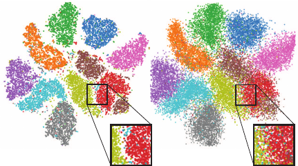
a) b)
Figure 1: Example of diffusion introduced by the NN pro-
jection. (a) Ground-truth t-SNE projection (b) Inferred NN
projection (10K samples). Insets show diffusion details.
However, this approach (further called Neural
Network (NN) projection for brevity) has two limi-
tations. First, and most seriously, the authors do not
show that learning occurs robustly, i.e., that the pre-
sented results are not singular cases due to lucky set-
tings of the many NN hyperparameters such as loss
function used, optimizer, regularization, or training-
set size. Deep learning is notoriously sensitive to
such settings, so fully exploring the NN hyperparam-
eter space is needed before one can make strong as-
sertions about the learning quality (Feurer and Hutter,
2019; Ilievski et al., 2017). This is especially impor-
tant for the DR approach in (Espadoto et al., 2019)
since, if this approach were indeed robust, it would
represent a major improvement to DR state-of-the-
art, given its simplicity, genericity, and speed. Sec-
ondly, it is visible from (Espadoto et al., 2019) that
the NN projections have some amount of diffusion,
i.e., they separate similar-sample clusters less clearly
than in a ground-truth t-SNE projection (see e.g. Fig-
ure 1). While visually salient, it is unclear how much
this diffusion affects the quality of a projection; and
how much this diffusion depends on hyperparameter
settings. Diffusion can have several causes, e.g.: (1)
underfitting, by training for too few epochs or having
too little data to learn from; (2) overfitting, by not hav-
ing proper regularization or also by having too little
data to learn from; (3) imperfect optimization, with
the optimizer getting stuck in local minima. How-
ever, which is the precise cause of diffusion is still
unknown and, thus, not controllable.
In this paper, we aim to answer both above issues
with the following contributions:
• we quantify the NN projection quality by using
four well-known projection quality metrics;
• we explore the hyperparameter space of NN pro-
jections, showing how these influence the results’
quality, gauged by the projection quality metrics;
• we show that NN projections are stable with re-
spect to hyperparameter settings, thereby com-
pleting the claim made by (Espadoto et al., 2019)
that they can be reliably used for out-of-sample
and noisy-data contexts.
The structure of this paper is as follows. Section 2
discusses related work on DR and neural networks.
Section 3 details our experimental setup. Section 4
presents our results, which are next discussed in Sec-
tion 5. Section 6 concludes the paper.
2 RELATED WORK
Related work can be split into dimensionality reduc-
tion and deep learning, as follows.
Dimensionality Reduction: Let x = (x
1
, . . . , x
n
), x
i
∈
R, 1 ≤ i ≤ n be an n-dimensional (nD) real-valued
sample, and let D = {x
i
}, 1 ≤ i ≤ N be a dataset of
N samples. Thus, D can be seen as a table with N
rows (samples) and n columns (dimensions). A pro-
jection technique is a function P : R
n
→ R
q
where
q n, and typically q = 2. The projection P(x) of
a sample x ∈ D is a 2D point. Projecting a set D
yields thus a 2D scatterplot, which we denote next as
P(D) = {P(x)|x ∈ D}.
Many Dimensionality Reduction (DR) techniques
have been developed over the years, with different
trade-offs of ease of use, scalability, distance preser-
vation, and out-of-sample capability. One of the
most widely used DR method is Principal Compo-
nent Analysis (Peason, 1901; Jolliffe, 1986) (PCA),
due to its ease of use and scalability. Manifold Learn-
ers, such as MDS (Torgerson, 1958), Isomap (Tenen-
baum et al., 2000) and LLE (Roweis and Saul, 2000)
try to reproduce in 2D the high-dimensional mani-
fold on which data is embedded, with the goal of
capturing nonlinear data structures. More recently,
UMAP (Uniform Manifold Approximation and Pro-
jection) (McInnes and Healy, 2018) was proposed,
based on simplicial complexes and manifold learning
techniques.
The SNE (Stochastic Neighborhood Embedding)
class of techniques, with t-SNE (van der Maaten and
Hinton, 2008) being its most successful member,
models similarity between samples as a probability
distribution of two points being neighbors of each
other, and try to reproduce the same probabilities in
2D. As outlined in Section 1, a key feature of t-SNE
is its ability to separate sample clusters very well in
visual space, which is very helpful for unsupervised
learning scenarios.
Deep Learning: Building well-performing neural
network (NN) architectures is very challenging due
to the many degrees of freedom allowed by their
design process. We outline below five typical such
degrees of freedom.
Network Architecture: Part of the power of NNs
comes from having many possible architectures, in
particular regarding number of layers and layer size,
if we restrict ourselves to fully-connected networks.
There is not a one-size-fits-all set of guidelines
to architecting NNs, which are typically created
empirically.
Regularization: NNs can be prone to overfitting,
which makes them fail to generalize during inference
for unseen data. Regularization techniques try to ad-
dress this by making the learning process harder, so
the NN can train for more epochs and generalize bet-
ter. Regularization techniques include L
2
, L
1
, max-
norm, early stopping, and data augmentation. The L
k
regularization techniques, also known as weight prun-
ing (k = 1) and weight decay (k = 2), work by adding
a penalization term of the form λkw
w
wk
k
to the NN loss
function, which equals the k-norm of the weights w
w
w
of a selected network layer. The parameter λ controls
the amount of regularization.
L
1
(Park and Hastie, 2007) regularization de-
creases layer weights with the less important getting
down to zero, leading to models with sparse weights.
L
2
(Krogh and Hertz, 1992) regularization decreases
layer weights to small but non-null values, leading to
models where every weight only slightly contributes
to the model. Both regularization techniques were ob-
served to help prevent overfitting. Max-norm (Srebro
and Shraibman, 2005), originally proposed for
Collaborative Filtering, was successfully applied
as a regularizer for NNs. It imposes a maximum
value γ for the norm of the layer weights. This
way, weight values are kept under control, similarly
to L
2
, but using a hard limit. Early stopping (Yao
et al., 2007) is a simple but effective way to prevent
overfitting, especially when combined with the other
regularization techniques outlined above. The idea
is to stop training when the training loss J
T
and
validation losses J
V
diverge, i.e., J
T
keeps decreasing
while J
V
stops decreasing or worse, starts increasing,
both of which signal overfitting.
Optimizers: Different optimizers are used for mini-
mizing the non-linear NN cost. The most used opti-
mizers are based on Mini-batch Stochastic Gradient
Descent (SGD) which is a variant of classic Gradi-
ent Descent (GD). GD aims to find optimal weights
w
w
w (that minimize the error created by the NN for the
training set) by adjusting these iteratively via the gra-
dient ∇J of the loss function J with respect to w
w
w as
w
w
w
t
= w
w
w
t−1
− η∇J (1)
where the learning rate η controls how large is each
update step t. Classic GD uses all data samples at
each iteration of Equation 1, which is costly for large
datasets. Stochastic Gradient Descent (SGD) alle-
viates this by using only one sample, picked ran-
domly, at each iteration. This speeds up computation
at the cost of having to solve a harder problem, as
there is less information available to the optimizer. A
commonly used optimizer today is Mini-batch SGD,
which uses one batch of samples for each GD itera-
tion, thus achieves a compromise between classic GD
and SGD. The Momentum method (Qian, 1999) im-
proves SGD convergence by adding to the update vec-
tor u
t
= η∇J at step t a fraction ν of the previous up-
date vector u
t−1
(Equation 2), i.e.
w
w
w
t
= w
w
w
t−1
− (νu
t−1
+ u
t
) (2)
However, tuning the learning rate η is not trivial:
Too small values may make the NN take too long
to converge; conversely, too high values may make
training miss good minima. Adaptive learning
optimizers, such as Adaptive Moment Estimation
(ADAM) (Kingma and Ba, 2014), alleviate this by
using squared gradients to compute the learning rate
dynamically. This greatly improves convergence
speed. However, (Wilson et al., 2017) found that
ADAM can find solutions that are worse than those
found by Mini-batch SGD. Solving this problem is
still an open research question.
Data Augmentation: Such techniques generate data
that are similar, but not identical, to existing training
data, to improve training when training-sets are
small. Such techniques highly depend on the data
type. Augmentation can be used for regularization
since adding more training data creates models that
generalize better.
Loss Functions: Finally, one needs to select an appro-
priate loss function J. For regression problems, com-
monly used loss functions are Mean Squared Error
(MSE), Mean Absolute Error (MAE), logcosh, and
Huber loss. Table 1 shows the definitions of these
functions, where
ˆ
y = { ˆy
i
} is the inferred output vec-
tor of the NN and y = {y
i
} is the training sample
ˆ
y
should match. MSE and logcosh are smoother func-
tions which are easier to optimize by GD or similar
methods outlined above. MAE is harder to optimize
since its gradient is constant. The Huber loss is some-
where in between the above, according to the param-
eter α: For values of α near zero, Huber behaves like
MAE; for larger α values, it behaves like MSE. MAE
and Huber losses are known to be more robust to out-
liers than MSE.
Table 1: Typical NN loss functions.
Function Definition
MSE
1
n
∑
n
i=1
(y
i
− ˆy
i
)
2
MAE
1
n
∑
n
i=1
|y
i
− ˆy
i
|
logcosh
1
n
∑
n
i=1
log(cosh(y
i
− ˆy
i
))
Huber
(
1
2
(y − ˆy)
2
if|y − ˆy| ≤ α
α|y − ˆy|−
1
2
α otherwise
Deep Learning Projections: The method proposed
in (Espadoto et al., 2019) uses deep learning to con-
struct projections as follows. Given a dataset D ⊂ R
n
,
a training subset D
t
⊂ D thereof is selected, and pro-
jected by a user-selected method (t-SNE or any other)
to yield a so-called training projection P(D
t
) ⊂ R
2
.
Next, D
t
is fed into a three-layer, fully-connected, re-
gression neural network which is trained to output a
2D scatterplot NN(D
t
) ⊂ R
2
by minimizing the mean
squared error between P(D
t
) and NN(D
t
). After that,
the network is used to construct projections of unseen
data by means of 2-dimensional, non-linear regres-
sion. Note that this approach is fundamentally dif-
ferent from autoencoders (Hinton and Salakhutdinov,
2006) which do not learn from a training projection
P, but simply aim to extract, in an unsupervised way,
latent low-dimensional features that best represent the
input data. The NN projection method is simple to im-
plement, generically learns any projection P for any
dataset D ⊂ R
n
, and is orders of magnitudes faster
than classical projection techniques, in particular t-
SNE. However, as outlined in Section 1, the quality
and stability of this method vs parameter setting has
not yet been assessed in detail. The goal of this pa-
per is to correct this important weakness of the work
in (Espadoto et al., 2019).
3 METHOD
3.1 Parameter Space Exploration
To achieve our objectives, listed in Section 1, we de-
signed and executed a set of experiments, detailed
next. For each experiment, we train and test the
NN projection with various combinations of datasets
and hyperparameter settings, and then interpret the
obtained results both quantitatively and qualitatively.
All parameter values used for each experiment are de-
tailed in this section. Early stopping was used on all
experiments, stopping training if the validation loss
stops decreasing for more than 10 epochs, and except
for the experiment with different optimizers, ADAM
was used on all experiments as well. As dataset,
we use MNIST (LeCun et al., 2010), which contains
70K samples of handwritten digits from 0 to 9, ren-
dered as 28x28-pixel grayscale images, flattened to
784-element vectors, with 10K test-set samples, and
varying training-set sizes of 2K, 5K, 10K and 20K
samples. We chose this dataset as it is complex, high-
dimensional, has a clear class separation, and it is well
known in dimensionality reduction literature. MNIST
was also used in (Espadoto et al., 2019), which makes
it easy to compare our results.
In line with the design choices available to NNs
outlined in Section 2, we explore the performance of
NN projections in the following directions.
Network Architecture (Section 4.5): We selected
three sizes of neural networks with 360 (small), 720
(medium) and 1440 (large) total number of units, and
distributed them into three different layouts, namely
straight (st), wide (wd) and bottleneck (bt), thus yield-
ing nine different architectures, as follows:
• Small - straight: 120, 120 and 120 units;
• Small - wide: 90, 180 and 90 units;
• Small - bottleneck: 150, 60 and 150 units;
• Medium - straight: 240, 240 and 240 units;
• Medium - wide: 180, 360 and 180 units;
• Medium - bottleneck: 300, 120 and 300 units;
• Large - straight: 480, 480 and 480 units;
• Large - wide: 360, 720 and 360 units;
• Large - bottleneck: 600, 240 and 600 units.
Besides these, we also tested the architecture
in (Espadoto et al., 2019), called next Standard,
which has three fully-connected hidden layers, with
256, 512, and 256 units respectively. All architec-
tures use ReLU activation functions, followed by a
2-element layer which uses the sigmoid activation
function to encode the 2D projection.
Regularization (Section 4.1): We explored the fol-
lowing regularization techniques:
• L
1
with λ ∈ {0, 0.001, 0.01, 0.1} with 0 meaning
no regularization;
• L
2
with λ ∈ {0, 0.001, 0.01, 0.1} with 0 meaning
no regularization;
• Max-norm constraint, with γ ∈ {0, 1, 2, 3}, with 0
meaning no constraint;
Optimizers (Section 4.2): We studied two optimiz-
ers: ADAM and Mini-batch SGD with learning rates
η ∈ {0.01, 0.001} and ν = 0.9. In both cases, we set
the batch size at 32 samples.

Data Augmentation (Section 4.3): We explored two
data augmentation strategies:
• Noise Before: We add Gaussian noise of zero
mean and different standard deviations σ ∈
{0, 0.001, 0.01}, with 0 meaning no noise, to the
high-dimensional training data, project this entire
(noise + clean samples) dataset, and ask the NN to
learn the projection. The idea is that, if the projec-
tion to learn (t-SNE in our case) can successfully
create well-separated clusters even for noisy data,
then our NN should learn how to do this as well;
• Noise After: We create the training projection
from clean data. We next add Gaussian noise
(same σ as before) to the data and train the NN to
project the entire (noise + clean samples) dataset
to the clean projection. The aim is to force the NN
to learn to project slightly different samples to the
same 2D point.
Loss Functions (Section 4.4): We studied four
types of loss functions: Huber, with parameters
α ∈ {1, 5, 10, 20, 30}; Mean Squared Error (MSE),
used by (Espadoto et al., 2019); Mean Absolute Error
(MAE); and logcosh.
Adding More Data: For all above directions, we
use different training-set sizes (2K, 5K, 10K and 20K
samples) to evaluate how this affects the results – that
is, how the NN projection quality depends on both
hyperparameter values and training-set size.
3.2 Quality Metrics
To evaluate the quality of the obtained projections,
we used the following four metrics well-known in the
DR literature (see Table 2). Of these, note that the
original paper (Espadoto et al., 2019) only discusses
Neighborhood Hit.
Trustworthiness T : Measures the fraction of points
in D that are also close in P(D) (Venna and Kaski,
2006). T tells how much one can trust that local
patterns in a projection, e.g. clusters, show actual
patterns in the data. U
(K)
i
is the set of points that are
among the K nearest neighbors of point i in the 2D
space but not among the K nearest neighbors of point
i in R
n
; and r(i, j) is the rank of the 2D point j in the
ordered set of nearest neighbors of i in 2D. We chose
K = 7 for this study, following (van der Maaten and
Postma, 2009; Martins et al., 2015);
Continuity C: Measures the fraction of points in
P(D) that are also close in D (Venna and Kaski,
2006). V
(K)
i
is the set of points that are among the K
nearest neighbors of point i in R
n
but not among the
K nearest neighbors in 2D; and ˆr(i, j) is the rank of
the R
n
point j in the ordered set of nearest neighbors
of i in R
n
. As in the case of T , we chose K = 7;
Neighborhood Hit NH: Measures how well-
separable labeled data is in a projection P(D)
from perfect separation (NH = 1) to no separation
(NH = 0) (Paulovich et al., 2008). NH equals the
number y
l
K
of the K nearest neighbors of a point
y ∈ P(D), denoted by y
K
, that have the same label as
y, averaged over P(D). In this paper, we used K = 7;
Shepard Diagram Correlation R: Shepard diagrams
are scatterplots of pairwise (Euclidean) distances be-
tween all points in P(D) vs corresponding distances
in D (Joia et al., 2011). Plots close to the main diago-
nal indicate better overall distance preservation. Plot
areas below, respectively above, the diagonal indicate
distance ranges for which false and missing neigh-
bors, respectively, occur. We measure the quality of a
Shepard diagram by computing its Spearman ρ rank
correlation. A value of R = 1 indicates a perfect (pos-
itive) correlation of distances.
Table 2: Quality metrics. Right column gives metric ranges,
with optimal values in bold.
Metric Definition
T 1 −
2
NK(2n−3K−1)
∑
N
i=1
∑
j∈U
(K)
i
(r(i, j) − K)
C 1 −
2
NK(2n−3K−1)
∑
N
i=1
∑
j∈V
(K)
i
(ˆr(i, j) − K)
NH
1
N
∑
y∈P(D)
y
l
k
y
k
R ρ(kx
i
− x
j
k, kP(x
i
) − P(x
j
)k), 1 ≤ i ≤ N, i 6= j
4 RESULTS
We next present the details of each experiment along
with the obtained results.
4.1 Regularization
We use increasing amounts of L
1
and L
2
regulariza-
tion to test if, by having a penalty term on the cost
function during training, the NN can generalize bet-
ter. We use L
1
and L
2
separately, to study how their
effects compare to each other.
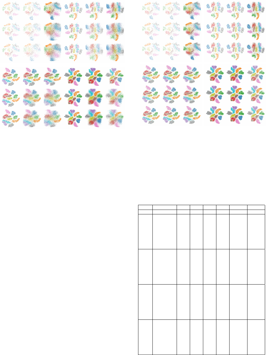
Figures 2 and 3 show the results. We see that, for
both L
1
and L
2
, the higher the regularization values
λ, the worse are the results. For instance, the result-
ing projection (train or test) becomes completely un-
related to the ground truth (training t-SNE projection)
when λ = 0.1. Separately, we see that L
2
regulariza-
tion performs better – that is, it produces projections
which are closer to the ground truth than the corre-
sponding projections produced using L
1
regulariza-
tion for the same λ values. Table 3 confirms the above
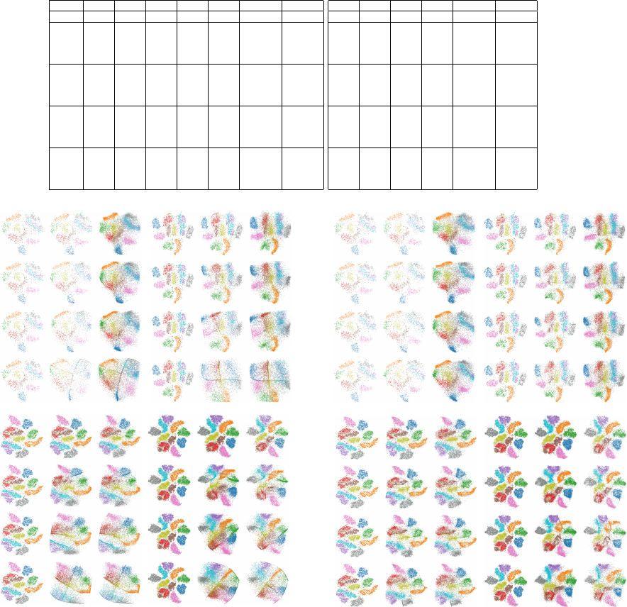
Table 3: Effect of regularization. Rows show metrics for t-SNE (GT row) vs NN projections using different training-set
sizes. Bold shows values closest to GT.
a) L
1
regularization
Model λ NH T C R # epochs Time (s)
GT 0.929 0.990 0.976 0.277
2K
0 0.705 0.843 0.957 0.443 50 6.20
0.001 0.677 0.827 0.948 0.439 58 7.14
0.01 0.660 0.815 0.945 0.438 94 10.93
0.1 0.632 0.806 0.943 0.454 82 9.98
5K
0 0.738 0.871 0.962 0.423 26 7.22
0.001 0.692 0.845 0.953 0.436 38 10.05
0.01 0.670 0.835 0.947 0.427 68 18.29
0.1 0.599 0.815 0.945 0.459 53 14.58
10K
0 0.834 0.902 0.968 0.337 45 22.32
0.001 0.753 0.852 0.958 0.348 31 16.09
0.01 0.722 0.833 0.951 0.352 39 19.12
0.1 0.665 0.811 0.947 0.345 61 30.67
20K
0 0.885 0.922 0.967 0.341 49 47.28
0.001 0.816 0.883 0.960 0.364 30 29.35
0.01 0.743 0.842 0.954 0.366 28 26.89
0.1 0.707 0.822 0.946 0.364 25 24.17
b) L
2
regularization
NH T C R # epochs Time (s)
0.929 0.990 0.976 0.277
0.695 0.839 0.956 0.437 35 4.61
0.711 0.847 0.958 0.432 29 4.27
0.684 0.834 0.954 0.433 42 5.57
0.683 0.830 0.952 0.428 68 8.54
0.767 0.880 0.963 0.422 53 14.33
0.742 0.875 0.963 0.419 28 7.71
0.733 0.866 0.959 0.416 55 15.24
0.709 0.860 0.958 0.429 45 12.51
0.833 0.899 0.967 0.342 43 20.93
0.821 0.899 0.966 0.340 55 27.88
0.798 0.880 0.963 0.337 34 17.37
0.773 0.865 0.961 0.336 36 18.48
0.885 0.922 0.967 0.341 46 43.49
0.870 0.915 0.966 0.343 34 33.06
0.853 0.902 0.963 0.344 40 38.05
0.826 0.883 0.960 0.339 38 37.87
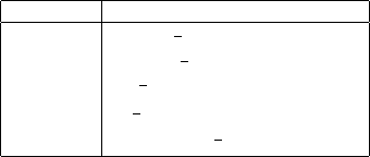
a) |T|=2K b) |T|=5K
c) |T|=10K d) |T|=20K
λ=0λ=0.001λ=0.01λ=0.1
λ=0λ=0.001λ=0.01λ=0.1
Training (t-SNE) Training (NN) Test (NN) Training (t-SNE) Training (NN) Test (NN)
Figure 2: L
1
regularization: Effect of λ for different
training-set sizes. Compare the ground truth (training-set,
projected by t-SNE) with the NN results on the training-set,
respectively test-set.
visual findings by showing quality metrics for the L
1
and L
2
regularization experiments. Overall, we see
that L
2
regularization produces NH, T , and C metrics
closer to the ground-truth (GT) values than L
1
reg-
ularization. This table also shows another interest-
ing insight: The NN projections yield higher Shepard
correlation R values than the ground truth t-SNE pro-
jection, for all regularization settings (slightly higher
for L
1
than L
2
). This tells us that the NN aims to
a) |T|=2K b) |T|=5K
c) |T|=10K d) |T|=20K
λ=0λ=0.001λ=0.01λ=0.1
λ=0λ=0.001λ=0.01λ=0.1
Training (t-SNE) Training (NN) Test (NN) Training (t-SNE) Training (NN) Test (NN)
Figure 3: L
2
regularization: Effect of λ for different
training-set sizes. Compare the ground truth (training-set,
projected by t-SNE) with the NN results on the training-set,
respectively test-set.
preserve the nD distances in the 2D projection more
than the t-SNE projection does (see definition of R,
Table 2). This explains, in turn, the diffusion we see
in the NN projections. In contrast, t-SNE does not
aim to optimize for distance preservation, but neigh-
borhood preservation, which results in a better cluster
separation but lower R values.
The rightmost two columns in Tables 3(a,b) show
the training effort needed for convergence (epochs
and seconds). We see that convergence is achieved for
all cases in under 70 epochs, regardless of the regular-
ization type (L
1
or L
2
) or strength λ. Also, L
1
and L
2
regularization have comparable costs, with L
2
being
slightly faster than L
1
for smaller training datasets.
Overall, the above tells us that the NN converges ro-
bustly regardless of regularization settings.
Table 4: Effect of max-norm. Metrics shown for t-SNE
(GT row) vs NN projections using different training-set
sizes. Bold shows values closest to GT.
Model γ NH T C R # epochs Time (s)
GT 0.929 0.990 0.976 0.277
2K
0 0.701 0.839 0.956 0.443 44 5.45
1 0.692 0.836 0.956 0.431 32 4.47
2 0.699 0.842 0.957 0.441 45 5.80
3 0.698 0.837 0.956 0.441 31 4.47
5K
0 0.759 0.881 0.964 0.417 51 13.34
1 0.756 0.880 0.964 0.421 40 10.70
2 0.740 0.866 0.961 0.420 24 7.05
3 0.755 0.879 0.963 0.423 48 13.23
10K
0 0.824 0.898 0.966 0.337 37 18.14
1 0.840 0.904 0.967 0.338 31 15.43
2 0.829 0.903 0.967 0.340 37 18.67
3 0.837 0.905 0.968 0.338 53 26.63
20K
0 0.886 0.923 0.967 0.342 56 52.65
1 0.870 0.918 0.967 0.340 26 25.22
2 0.881 0.917 0.967 0.341 30 28.88
3 0.879 0.920 0.967 0.345 34 34.11
Next, we study max-norm regularization, to see
how this affects the NN generalization capability. Fig-
ure 4 shows that the projection quality is not strongly
dependent on γ, and the metrics in Table 4 confirm
this. More importantly, we see that max-norm yields
projections which are better in terms of all quality
metrics than L
1
and L
2
regularization, and closer to
the t-SNE ground truth. Effort-wise, max-norm regu-
larization is very similar to L
1
and L
2
(compare right-
most columns in Table 4 with those in Table 3(a,b)).
In conclusion, for this particular problem we deter-
mine that regularization brings no clear benefit.
4.2 Optimizer
The quality of the NN projection obviously depends
on how well the optimization method used during
training can minimize the cost function (Section 2).
To find out how the projection quality is influenced
by optimization choices, we trained the NN using the
ADAM optimizer with its default settings, and also
with SGD with learning rates η ∈ {0.01, 0.001}. Fig-
ure 5 shows that the ADAM optimizer produces re-
sults with considerably less diffusion than SGD. Ta-
ble 5 clearly confirms this, as ADAM scores bet-
ter than SGD for all considered quality metrics. We
also see here that ADAM converges much faster than
SGD. Since, additionally, ADAM works well with its
default parameters, we conclude that this is the opti-
mizer of choice for our problem.
a) |T|=2K b) |T|=5K
c) |T|=10K d) |T|=20K
no max normγ=1.0γ=2.0γ=3.0
Training (t-SNE) Training (NN) Test (NN) Training (t-SNE) Training (NN) Test (NN)
no max normγ=1.0γ=2.0γ=3.0
Figure 4: Max-norm: Effect of γ for different training-set
sizes. Compare the ground truth (training-set, projected by
t-SNE) with the NN results on the training-set, respectively
test-set.
Table 5: Effect of optimizers. Metrics shown for t-SNE
(GT row) vs NN projections using different training-set
sizes. Bold shows values closest to GT.
Model Optimizer (η) NH T C R # epochs Time (s)
GT 0.929 0.990 0.976 0.277
2K
ADAM 0.696 0.841 0.956 0.447 30 3.72
SGD (0.01) 0.625 0.791 0.938 0.464 97 8.32
SGD (0.001) 0.610 0.787 0.938 0.464 455 36.56
5K
ADAM 0.733 0.861 0.960 0.421 19 5.27
SGD (0.01) 0.655 0.817 0.945 0.439 86 16.90
SGD (0.001) 0.641 0.808 0.942 0.443 402 77.17
10K
ADAM 0.842 0.905 0.968 0.343 56 26.51
SGD (0.01) 0.707 0.821 0.949 0.362 75 28.55
SGD (0.001) 0.690 0.812 0.948 0.360 392 147.60
20K
ADAM 0.882 0.920 0.968 0.339 43 40.77
SGD (0.01) 0.769 0.838 0.952 0.356 129 94.30
SGD (0.001) 0.754 0.836 0.952 0.370 423 309.19
4.3 Noise-based Data Augmentation
Here we turn to data augmentation to try to address
the problem of reducing diffusion in the NN projec-
tion. For this, we add noise to the data as described
in Section 3.1 to observe if it improves learning. Fig-
ures 6 and 7 show that both the Noise before and Noise
after strategies produce quite similar results, which
are also close to the ground truth. Table 7(a,b) con-
firms this, additionally showing that the Noise after
strategy yields slightly higher quality metrics on aver-
a) |T|=2K b) |T|=5K
c) |T|=10K d) |T|=20K
ADAMSGD η=0.01
Training (t-SNE) Training (NN) Test (NN) Training (t-SNE) Training (NN) Test (NN)
SGD η=0.001
ADAMSGD η=0.01
SGD η=0.001
Figure 5: Optimizer: Effects of different settings (ADAM,
SGD with η ∈ {0.001, 0.01}) for different training-set sizes.
Compare the ground truth (training-set, projected by t-SNE)
with the NN results on the training-set, respectively test-set.
age than Noise before. More importantly, if we com-
pare these values with those obtained by trying dif-
ferent regularization techniques and optimizers (Ta-
bles 3-4), we see that Noise after slightly improves
the projection quality.
4.4 Loss Function
Next we study the effect of using different loss func-
tions. Figure 8 shows that MAE produces visual clus-
ters that are slightly sharper than the ones created with
the other loss functions studied. Also, we see that this
effect is more pronounced on tests with lower num-
bers of training samples. This effect is confirmed by
looking at the quality metrics in Table 6: For instance,
using MAE yields an increase of NH from roughly
0.70 (when using the other loss functions) to roughly
0.74 for the smallest test-set of 2K samples; for the
largest test-set of 20K samples, the comparable NH
increase is from roughly 0.87 to 0.88. Still, MAE
achieves consistently the best quality metrics for al-
most all the tested cases, as compared to using the
other loss functions. Separately, we see in Table 6
that the training effort for MAE is higher than when
using the other loss functions. However, as the num-
ber of samples increases, the training-effort difference
decreases, which is important, as it tells us that, for
realistic (larger training-sets) cases, using MAE is not
really costing more than using other loss functions.
a) |T|=2K b) |T|=5K
c) |T|=10K d) |T|=20K
no noiseσ=0.001
Training (t-SNE) Training (NN) Test (NN) Training (t-SNE) Training (NN) Test (NN)
σ=0.01
no noiseσ=0.001
σ=0.01
Figure 6: Noise after data augmentation: Effect of noise
strength σ ∈ {0, 0.001, 0.01}. Compare the ground truth
(training-set, projected by t-SNE) with the NN results on
the training-set, respectively test-set.
Given the quality increase, we conclude that MAE is
the best loss function.
Table 6: Effect of different loss functions. Rows show met-
rics for t-SNE (GT row) vs NN projections using different
training-set sizes. Bold shows values closest to GT.
Model Loss (α) NH T C R # epochs Time (s)
GT 0.929 0.990 0.976 0.277
2K
Huber (1.0) 0.706 0.839 0.956 0.445 34 5.94
Huber (5.0) 0.687 0.827 0.953 0.447 16 3.99
Huber (10.0) 0.704 0.839 0.957 0.431 45 7.53
Huber (20.0) 0.692 0.835 0.956 0.442 32 5.88
Huber (30.0) 0.695 0.836 0.956 0.433 30 5.98
logcosh 0.704 0.839 0.957 0.434 33 6.37
MAE 0.742 0.866 0.962 0.423 78 11.05
MSE 0.704 0.842 0.957 0.442 40 6.86
5K
Huber (1.0) 0.762 0.883 0.964 0.420 50 14.50
Huber (5.0) 0.745 0.871 0.963 0.426 26 8.34
Huber (10.0) 0.769 0.886 0.965 0.416 69 19.79
Huber (20.0) 0.763 0.884 0.965 0.420 62 18.18
Huber (30.0) 0.768 0.883 0.965 0.420 55 16.16
logcosh 0.768 0.883 0.965 0.425 54 16.03
MAE 0.781 0.893 0.965 0.418 57 16.56
MSE 0.753 0.874 0.963 0.428 30 9.67
10K
Huber (1.0) 0.831 0.898 0.968 0.338 38 19.56
Huber (5.0) 0.833 0.902 0.968 0.342 40 20.64
Huber (10.0) 0.837 0.906 0.969 0.344 52 26.98
Huber (20.0) 0.831 0.900 0.968 0.344 38 19.97
Huber (30.0) 0.831 0.902 0.968 0.348 36 19.55
logcosh 0.818 0.893 0.967 0.347 25 14.00
MAE 0.848 0.912 0.968 0.333 58 29.55
MSE 0.839 0.906 0.968 0.339 65 32.42
20K
Huber (1.0) 0.856 0.907 0.967 0.353 20 19.57
Huber (5.0) 0.881 0.918 0.967 0.344 44 41.69
Huber (10.0) 0.882 0.921 0.968 0.344 36 34.48
Huber (20.0) 0.881 0.920 0.967 0.342 45 43.96
Huber (30.0) 0.877 0.915 0.967 0.341 29 28.71
logcosh 0.884 0.919 0.967 0.335 35 35.46
MAE 0.887 0.927 0.966 0.339 47 44.55
MSE 0.871 0.914 0.967 0.341 23 21.68
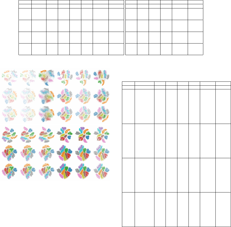
Table 7: Effect of data augmentation. Rows show metrics for t-SNE (GT row)) vs NN projections (other rows). Right two
columns in each table show training effort (epochs and time). Bold shows values closest to GT.
a) Noise after strategy
Model Noise σ NH T C R # epochs Time (s)
GT 0.929 0.990 0.976 0.277
2K
0 0.717 0.846 0.958 0.448 31 8.84
0.001 0.726 0.852 0.960 0.430 37 10.57
0.01 0.729 0.856 0.960 0.433 54 14.52
5K
0 0.783 0.892 0.966 0.401 43 23.28
0.001 0.780 0.895 0.966 0.408 52 29.44
0.01 0.783 0.892 0.966 0.401 47 26.84
10K
0 0.849 0.909 0.968 0.339 44 44.06
0.001 0.844 0.909 0.968 0.337 36 37.76
0.01 0.848 0.910 0.968 0.333 59 60.31
20K
0 0.887 0.924 0.966 0.340 55 105.87
0.001 0.888 0.924 0.967 0.336 46 88.09
0.01 0.885 0.925 0.967 0.339 51 97.06
b) Noise before strategy
NH T C R # epochs Time (s)
0.929 0.990 0.976 0.277
0.712 0.842 0.957 0.446 23 7.17
0.679 0.842 0.959 0.422 33 9.57
0.682 0.833 0.956 0.421 20 6.86
0.785 0.894 0.966 0.401 62 33.34
0.793 0.884 0.966 0.364 31 17.91
0.802 0.888 0.967 0.366 49 28.68
0.849 0.908 0.968 0.336 36 35.61
0.798 0.901 0.966 0.304 37 39.58
0.802 0.904 0.966 0.302 53 55.58
0.888 0.925 0.967 0.337 40 76.08
0.865 0.920 0.967 0.385 42 81.55
0.869 0.920 0.967 0.392 41 80.52
a) |T|=2K b) |T|=5K
c) |T|=10K d) |T|=20K
no noiseσ=0.001
Training (t-SNE) Training (NN) Test (NN) Training (t-SNE) Training (NN) Test (NN)
σ=0.01
no noiseσ=0.001
σ=0.01
Figure 7: Noise before data augmentation: Effect of noise
strength σ ∈ {0, 0.001, 0.01}. Compare the ground truth
(training-set, projected by t-SNE) with the NN results on
the training-set, respectively test-set.
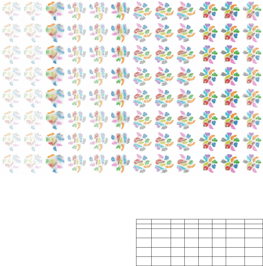
4.5 Network Architecture
Finally, we study the effect of using different NN
architectures. Figure 9 shows that the architecture
Large - bottleneck produces visual clusters that are
slightly sharper than the ones created by the other ar-
chitectures studied. This is confirmed by the quality
metrics in Table 8: We see that Large - bottleneck
has a NH about 0.04 higher for all training-set sizes.
Also, while this architecture is larger than the others,
its training effort is quite similar to that of the other
architectures.
Table 8: Effect of different NN Architectures. Rows show
metrics for t-SNE (GT row) vs NN projections using differ-
ent training-set sizes. Bold shows values closest to GT.
Model NN Arch NH T C R # epochs Time (s)
GT 0.929 0.990 0.976 0.277 0 0
2K
small st 0.680 0.827 0.951 0.437 30 5.11
small bt 0.670 0.819 0.950 0.453 18 3.85
small wd 0.672 0.820 0.949 0.463 17 3.82
medium st 0.683 0.827 0.952 0.441 17 3.83
medium bt 0.690 0.833 0.955 0.456 25 4.96
medium wd 0.702 0.838 0.956 0.438 44 7.17
large st 0.692 0.835 0.956 0.447 19 4.66
large bt 0.720 0.852 0.961 0.430 50 8.95
large wd 0.713 0.847 0.959 0.434 45 8.30
5K
small st 0.744 0.875 0.962 0.414 66 18.31
small bt 0.719 0.855 0.958 0.423 17 5.78
small wd 0.726 0.864 0.959 0.424 40 12.21
medium st 0.761 0.879 0.963 0.418 42 12.67
medium bt 0.742 0.872 0.962 0.426 33 10.54
medium wd 0.740 0.873 0.963 0.419 40 12.53
large st 0.752 0.874 0.964 0.408 29 10.95
large bt 0.761 0.880 0.964 0.420 34 12.02
large wd 0.755 0.878 0.964 0.423 38 13.87
10K
small st 0.818 0.893 0.966 0.338 43 21.02
small bt 0.820 0.893 0.966 0.330 54 27.35
small wd 0.794 0.879 0.963 0.330 28 15.35
medium st 0.828 0.900 0.968 0.343 45 22.74
medium bt 0.820 0.895 0.967 0.343 31 16.68
medium wd 0.825 0.899 0.967 0.338 49 25.74
large st 0.831 0.902 0.968 0.338 32 20.34
large bt 0.836 0.905 0.969 0.341 36 21.97
large wd 0.830 0.900 0.968 0.338 30 19.31
20K
small st 0.865 0.910 0.965 0.335 30 30.81
small bt 0.838 0.891 0.965 0.353 16 15.74
small wd 0.865 0.910 0.965 0.345 37 34.66
medium st 0.882 0.922 0.967 0.339 45 41.97
medium bt 0.882 0.921 0.967 0.340 45 41.35
medium wd 0.874 0.917 0.967 0.346 34 32.92
large st 0.886 0.924 0.967 0.340 45 50.74
large bt 0.890 0.925 0.967 0.342 37 42.48
large wd 0.878 0.917 0.967 0.345 29 33.03
5 DISCUSSION
We next summarize the obtained insights, as follows.
Optimal Settings: Our experiments showed that the
proposed NN projection attains optimal quality (and
closest to the ground-truth t-SNE projection) with
no regularization, ADAM optimizer, Noise after data
augmentation, MAE loss function, and Large - Bot-
tleneck architecture. The choice of σ (noise standard
deviation for data augmentation) affects very little the
measured quality, so one should not be concerned in
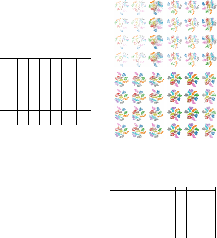
Training (t-SNE) Training (NN) Test (NN)
a) |T|=2K
Training (t-SNE) Training (NN) Test (NN)
b) |T|=5K
Training (t-SNE) Training (NN) Test (NN)
c) |T|=10K
Training (t-SNE) Training (NN) Test (NN)
d) |T|=10K
Huber α=1Huber α=5Huber α=10Huber α=20Huber α=30MSEMAElogcosh
Figure 8: Loss: Effect of different loss functions. Compare the ground truth (training-set, projected by t-SNE) with the NN
results on the training-set, respectively test-set.
practice by how to set this parameter.
Given the above optimal settings, with σ = 0.01,
we did one last experiment to evaluate how they
perform when combined. We ran both the original
Std architecture and the Large - Bottleneck, both
using the optimal settings, to better assess the effect
of the architecture change. In Table 9 we see that
Large - Bottleneck performs better than Std on
practically all metrics and for all training-set sizes.
This improvement can be seen even when compared
to the best results of each individual test, especially
for smaller training-set sizes. Figure 10 shows this
improvement in the form of less fuzziness and better
separated clusters.
Quality: We have measured four well-known pro-
jection quality metrics: neighborhood hit, trustwor-
thiness, continuity, and Shepard diagram correlation.
Our experiments show that all these metrics are stable
with respect to hyperparameter settings. More impor-
tantly, the optimal setting outlined above yields val-
ues which are very close to the ground-truth t-SNE
values, and actually closer to ground-truth than the
results presented in (Espadoto et al., 2019). As the
training-set increases in size, the NN quality metrics
Table 9: Effect of using optimal settings. Metrics shown
for t-SNE (GT row) vs NN projections using different
training-set sizes. Bold shows values closest to GT.
Model NN Arch NH T C R # epochs Time (s)
GT 0.929 0.990 0.976 0.277 0 0
2K
std 0.753 0.871 0.963 0.433 73 14.58
large bt 0.773 0.878 0.964 0.426 82 18.44
5K
std 0.794 0.904 0.964 0.411 129 60.26
large bt 0.813 0.906 0.966 0.411 70 37.19
10K
std 0.850 0.916 0.967 0.334 113 104.39
large bt 0.850 0.913 0.966 0.331 108 112.53
20K
std 0.884 0.923 0.964 0.335 121 215.66
large bt 0.891 0.929 0.964 0.335 101 205.07
consistently approach the ground-truth values – see
Tables 3-8 for training-sets from 2K to 20K samples.
The difference of the two is under 5% on average for
training-sets of 20K points. We believe that this dif-
ference is a quite acceptable accuracy loss, given the
simplicity, genericity, and high speed of the NN pro-
jection (all these aspects having been discussed in de-
tail in (Espadoto et al., 2019)).
Visual examination of the NN projections shows
that these exhibit a discernible amount of diffusion
as compared to the ground-truth t-SNE projections.
While diffusion clearly decreases with training-set
size, it is still present even for the optimal parame-
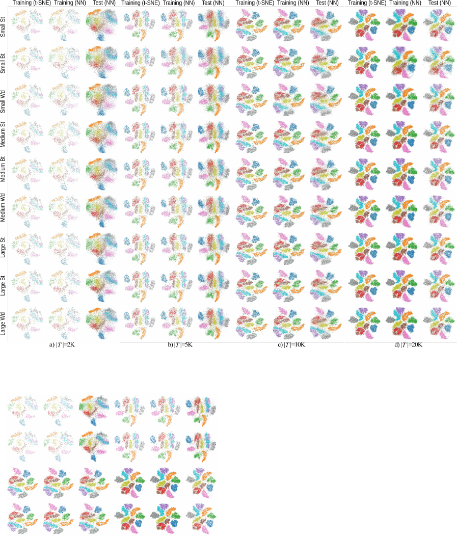
Figure 9: NN Arch: Effect of different NN Architectures. Compare the ground truth (training-set, projected by t-SNE) with
the NN results on the training-set, respectively test-set.
Training (t-SNE) Training (NN) Test (NN)
Training (t-SNE) Training (NN) Test (NN)
a) |
T
|=2K
b) |
T
|=5K
c) |
T
|=10K
d) |
T
|=20K
Large Bt
Std
Large Bt
Std
Figure 10: Optimal Settings: Effect of using optimal set-
tings for Std and Large - Bottleneck NN architectures. Com-
pare the ground truth (training-set, projected by t-SNE) with
the NN results on the training-set, respectively test-set.
ter settings and 20K training samples – compare e.g.
the inference on unseen data in Figure 7(d, test (NN))
with Figure 7(d, training, t-SNE).
Stability: An important result of our experiments is
that the NN projection method is stable with respect
to training-set sizes, hyperparameter settings, noise
and loss functions. Indeed, Figures 2-9 show, re-
gardless from the already discussed diffusion effect,
practically the same shape and relative positions
of the data clusters in the test projections (NN
method run on unseen data) and the ground-truth
t-SNE projections, for all tested configurations.
The stability of the NN projection with respect to
training data, parameter settings, and noise is in
stark contrast with the instability of the ground-truth
t-SNE projection with respect to all these three
factors, and is of important practical added-value in
many applications (Wattenberg, 2016).
Improving Projections: Following our analysis, the
only noticeable drawback we see for the NN projec-
tions is the already discussed diffusion. Indeed, the
main advantage of t-SNE praised by basically all its
users is its ability to strongly separate similar-value
sample clusters. Our experiments show that the NN
projection can reach similar, though not fully identi-
cal, separation levels. Two open questions arise here:
(1) How can we adapt the NN approach to learn such
a strong separation? Our experiments show that hy-
perparameter settings, including regularization, data
augmentation, optimizer, loss function and network
architecture cannot fully eliminate diffusion, although
by using MAE as loss function, quality metrics in-
creased in value. The main open dimension to study
is using non-standard loss functions than those used;
(2) Can we design quality metrics able to better cap-
ture diffusion? If so, such metrics could be used to
next design suitable loss functions to minimize this
undesired effect. Both these issues are open to future
research.
6 CONCLUSION
We presented an in-depth study aimed at assessing the
quality and stability of dimensionality reduction (DR)
using supervised deep learning. For this, we explored
the design space of a recent deep learning method
in this class (Espadoto et al., 2019) in six orthogo-
nal directions: training-set size, network architecture,
regularization, optimization, data augmentation, and
loss functions. These are the main design degrees-
of-freedom present when creating any deep learning
architecture. We sampled each direction using sev-
eral settings (method types and parameter values) and
compared the resulting projections with the ground-
truth (t-SNE method) quantitatively, using four qual-
ity metrics, and also qualitatively by visual inspec-
tion.
Our results deliver an optimal hyperparameter set-
ting for which the deep-learned projections can ap-
proach very closely the quality of the t-SNE ground
truth. Separately, we showed that the deep learning
projection method is stable with respect to all param-
eter settings, training-set size, and noise added to the
input data. These results complement recent evalua-
tions (Espadoto et al., 2019) to argue strongly that su-
pervised deep learning is a practical, robust, simple-
to-set-up, and high-quality alternative to t-SNE for
dimensionality reduction in data visualization. More
broadly, this study is, to our knowledge, the only work
that presents in detail how hyperparameter spaces of a
projection method can be explored to find optimal set-
tings and evidence for the projection method stability.
We believe that our methodology can be directly used
to reach the same goals (optimal settings and proof
of stability) for any projection technique under study,
whether using deep learning or not.
We plan to extend these results in several direc-
tions. First, we aim to explore non-standard loss func-
tions to reduce the small, but visible, amount of dif-
fusion present in the deep learned projections. Sec-
ondly, we aim to extend our approach to project time-
dependent data in a stable and out-of-sample manner,
which is a long-standing, but not yet reached, goal for
high-dimensional data visualization.
ACKNOWLEDGMENTS
This study was financed in part by the Coordenac¸
˜
ao
de Aperfeic¸oamento de Pessoal de N
´
ıvel Superior -
Brasil (CAPES) - Finance Code 001.
REFERENCES
Espadoto, M., Hirata, N., and Telea, A. (2019). Deep learn-
ing multidimensional projections. arXiv:1902.07958
[cs.CG].
Feurer, M. and Hutter, F. (2019). Hyperparameter optimiza-
tion. In Automated Machine Learning. Springer.
Hinton, G. E. and Salakhutdinov, R. R. (2006). Reducing
the dimensionality of data with neural networks. Sci-
ence, 313(5786):504–507.
Ilievski, I., Akhtar, T., Feng, J., and Shoemaker, C. (2017).
Efficient hyperparameter optimization of deep learn-
ing algorithms using deterministic RBF surrogates. In
Proc. AAAI.
Joia, P., Coimbra, D., Cuminato, J. A., Paulovich, F. V., and
Nonato, L. G. (2011). Local affine multidimensional
projection. IEEE TVCG, 17(12):2563–2571.
Jolliffe, I. T. (1986). Principal component analysis and fac-
tor analysis. In Principal Component Analysis, pages
115–128. Springer.
Kehrer, J. and Hauser, H. (2013). Visualization and vi-
sual analysis of multifaceted scientific data: A survey.
IEEE TVCG, 19(3):495–513.
Kingma, D. and Ba, J. (2014). Adam: A method for
stochastic optimization. arXiv:1412.6980.
Krogh, A. and Hertz, J. A. (1992). A simple weight decay
can improve generalization. In NIPS, pages 950–957.
LeCun, Y., Cortes, C., and Burges, C. (2010).
MNIST handwritten digit database. AT&T Labs
http://yann.lecun.com/exdb/mnist, 2.
Liu, S., Maljovec, D., Wang, B., Bremer, P.-T., and
Pascucci, V. (2015). Visualizing high-dimensional
data: Advances in the past decade. IEEE TVCG,
23(3):1249–1268.
Martins, R., Minghim, R., and Telea, A. C. (2015). Explain-
ing neighborhood preservation for multidimensional
projections. In Proc. CGVC, pages 121–128. Euro-
graphics.
McInnes, L. and Healy, J. (2018). UMAP: Uniform man-
ifold approximation and projection for dimension re-
duction. arXiv:1802.03426.
Nonato, L. and Aupetit, M. (2018). Multidimensional
projection for visual analytics: Linking techniques
with distortions, tasks, and layout enrichment. IEEE
TVCG.
Park, M. Y. and Hastie, T. (2007). L1-regularization path
algorithm for generalized linear models. J Royal Stat
Soc: Series B, 69(4):659–677.
Paulovich, F. V., Nonato, L. G., Minghim, R., and Lev-
kowitz, H. (2008). Least square projection: A fast
high-precision multidimensional projection technique
and its application to document mapping. IEEE
TVCG, 14(3):564–575.
Peason, K. (1901). On lines and planes of closest fit to
systems of point in space. Philosophical Magazine,
2(11):559–572.
Qian, N. (1999). On the momentum term in gradi-
ent descent learning algorithms. Neural networks,
12(1):145–151.
Rauber, P., Falc
˜
ao, A. X., and Telea, A. (2016). Visualizing
time-dependent data using dynamic t-SNE. In Proc.
EuroVis: Short Papers, pages 73–77.
Roweis, S. T. and Saul, L. K. (2000). Nonlinear dimension-
ality reduction by locally linear embedding. Science,
290(5500):2323–2326.
Srebro, N. and Shraibman, A. (2005). Rank, trace-norm and
max-norm. In Intl. Conf. on Computational Learning
Theory, pages 545–560. Springer.
Tenenbaum, J. B., De Silva, V., and Langford, J. C. (2000).
A global geometric framework for nonlinear dimen-
sionality reduction. Science, 290(5500):2319–2323.
Torgerson, W. (1958). Theory and Methods of Scaling. Wi-
ley.
van der Maaten, L. and Hinton, G. E. (2008). Visualizing
data using t-SNE. JMLR, 9:2579–2605.
van der Maaten, L. and Postma, E. (2009). Dimensionality
reduction: A comparative review. Technical report,
Tilburg Univ., Netherlands. TiCC 2009-005.
Venna, J. and Kaski, S. (2006). Visualizing gene interaction
graphs with local multidimensional scaling. In Proc.
ESANN, pages 557–562.
Wattenberg, M. (2016). How to use t-SNE effectively.
https://distill.pub/2016/misread-tsne.
Wilson, A., Roelofs, R., Stern, M., Srebro, N., and Recht,
B. (2017). The marginal value of adaptive gradient
methods in machine learning. In NIPS, pages 4148–
4158.
Yao, Y., Rosasco, L., and Caponnetto, A. (2007). On early
stopping in gradient descent learning. Constructive
Approximation, 26(2):289–315.
