
A Hierarchical Convolution Neural Network Scheme for Radar Pulse
Detection
Van Long Do, Ha Phan Khanh Nguyen, Dat Thanh Ngo and Ha Quy Nguyen
Viettel High Technology Industries Corporation, Hoa Lac High-tech Park, Hanoi, Vietnam
Keywords:
Deep Learning, Hierarchical Neural Network, Radar Pulse Detection, Denoising Neural Network.
Abstract:
The detection of radar pulses plays a critical role in passive radar systems since it provides inputs for other
algorithms to localize and identify emitting targets. In this paper, we propose a hierarchical convolution
neural network (CNN) to detect narrowband radar pulses of various waveforms and pulse widths at different
noise levels. The scheme, named DeepIQ, takes a fixed-length segment of raw IQ samples as inputs and
estimates the time of arrival (TOA) and the time of departure (TOD) of the radar pulse, if any, appearing
in the segment. The estimated TOAs and TODs are then combined across segments to form a sequential
detection mechanism. The DeepIQ scheme consists of sub-networks performing three different tasks: segment
classification, denoising and edge detection. The proposed scheme is a full deep learning-based solution and
thus, does not require any noise floor estimation process, as opposed to the commonly used Threshold-based
Edge Detection (TED) methods. Simulation results show that the proposed solution significantly outperforms
other schemes, especially under severe noise levels.
1 INTRODUCTION
In passive radar systems (Torrieri, 1984; Poisel,
2005), for example, Electronic Intelligence (ELINT)
or Early Warning System (EWS), the detection of
radar pulses is the process of estimating pairs of
the time of arrival (TOA) and the time of departure
(TOD) of the pulses from a sequence of received I/Q
samples. This task is essential for the location and
identification of emitting sources. However, this is
not a trivial problem. Nowadays, radar signals are
very diversified with various modulation types and
pulse widths (Levanon and Mozeson, 2004; Richards,
2014; Pace, 2009). Moreover, in severe conditions
with low Signal–to–Noise Ratio (SNR) level, most of
radar pulses are buried in noise. Therefore, it is very
difficult to detect the presence of true radar pulses in
such noisy environments.
In recent years, Deep Learning (LeCun et al.,
2015; Goodfellow et al., 2016) has emerged as
a powerful tool for many tasks in computer vi-
sion and image processing such as image classifica-
tion (Krizhevsky et al., 2012; Szegedy et al., 2015; He
et al., 2016), denoising and image restoration (Zhang
et al., 2017; Mao et al., 2016), and object detec-
tion (Ren et al., 2017; Redmon et al., 2016; Liu et al.,
2016). Inspired by these successes, in this paper, we
focus on designing a full deep learning-based scheme,
named DeepIQ, for radar pulse detection. In this
method, the received radar signal is first divided into
overlapping fixed-length segments, each of which is
then fed to a hierarchical convolutional neural net-
work to estimate the TOA and/or TOD, if any. By
using sufficiently small segments, we can safely as-
sume that each segment contains at most one radar
pulse. The TOA and TOD estimates obtained from
DeepIQ are tracked and updated, if necessary, after
each segment is processed.
The contribution of this paper is as follows:
• We present a novel neural network structure,
called Classification Net to determine whether a
radar pulse appears in the segment. By using
deep-learning based approach, we get rid of noise
floor estimation process for setting the detection
threshold as in previous works.
• We design a denoising neural network, named De-
noising Net to mitigate the noise effect on re-
ceived radar signal and thus improve significantly
the detection accuracy.
• We propose a neural network architecture, named
Edge-Detection Net, which contains three differ-
ent nets (TOA Net, TOD Net and TOA-TOD Net)
with the same architecture to estimate the TOA
Do, V., Nguyen, H., Ngo, D. and Nguyen, H.
A Hierarchical Convolution Neural Network Scheme for Radar Pulse Detection.
DOI: 10.5220/0008876500150022
In Proceedings of the 9th International Conference on Pattern Recognition Applications and Methods (ICPRAM 2020), pages 15-22
ISBN: 978-989-758-397-1; ISSN: 2184-4313
Copyright
c
2022 by SCITEPRESS – Science and Technology Publications, Lda. All rights reserved
15
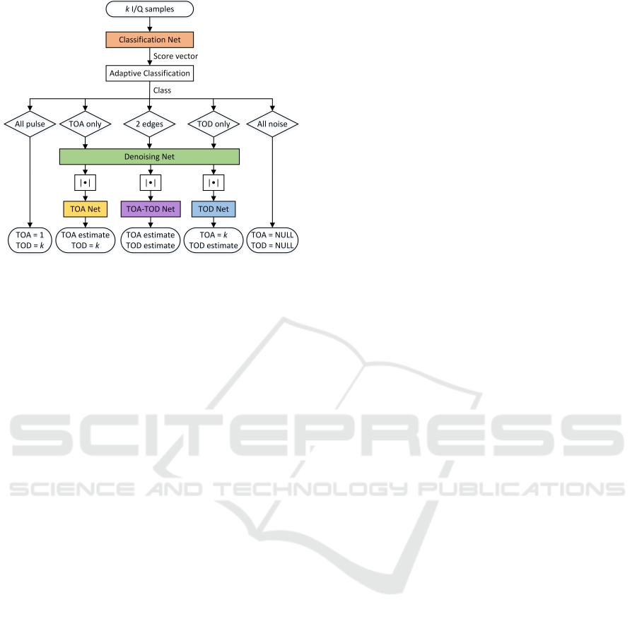
Figure 1: Flowchart of the DeepIQ network.
and/or TOD from the received radar signal de-
pending on the result of the Classification Net.
• We conduct extensive simulations to evaluate the
effectiveness of our proposed scheme. The simu-
lation results indicate that DeepIQ improves sig-
nificantly the radar pulse detection accuracy.
Figure 1 depicts the overview of the DeepIQ
scheme. The proposed method receives a segment
of k I/Q samples and estimates the TOA and TOD
of radar pulses. Our proposed CNN blocks are high-
lighted in colored. The symbol | · | denotes the modu-
lus operator.
The rest of this paper is organized as follows. We
first review the related studies in Section II. In Sec-
tion III, we describe necessary assumptions and for-
mally define the problem. The detail of our proposed
scheme is shown in Section IV. We show simulation
results in Section V. Finally, the conclusion is pre-
sented in Section VI.
2 RELATED WORK
Since radar pulse detection is an important opera-
tion in Electronic Warfare systems such as ELINT or
EWS, there are many studies on this problem in re-
cent years. In (Torrieri, 1974; Iglesias et al., 2014),
the authors proposed an adaptive thresholding scheme
to detect and estimate the TOA and TOD of radar
pulses. Albaker et al. (Albaker and Rahim, 2011) ap-
plied a dual threshold noise gate subsystem to ex-
tract the parameters of radar pulses. The authors
in (Lakshmi et al., 2013) proposed a model for de-
tection and extraction of pulse parameters in Radar
Warning Receivers. In their model, the TOA and
TOD are estimated by a predefined hard threshold.
In (Lancon et al., 1996), the radar signal is extracted
using a correlation method that takes advantage of
the periodic characteristic of radar signals. In this
method, a detection threshold is selected to determine
the correlation peak based on the noise statistic. To
the best of our knowledge, all of the aforementioned
schemes for radar pulse detection are threshold-based,
in which the thresholds are defined through estimat-
ing the noise statistics. These methods yield good
performances under high or moderate SNR levels but
fail under low SNR levels. Moreover, the noise floor
estimation–an essence of these algorithms–is itself a
non-trivial task, especially in quickly varying envi-
ronments.
In our previous work (Nguyen et al., 2019), we
introduced a deep learning based framework to solve
radar pulse detection problem. The method consists
of two steps. In the first step, a CNN is trained to
determine whether a pulse or part of a pulse appears
in a segment of the signal. In the second step, TOA
and TOD of radar pulses are estimated by finding the
change points in the segment via Pruned Exact Lin-
ear Time (PELT) method (Killick et al., 2012). Al-
though this method improved significantly the radar
pulse detection performance in comparison with other
TED methods, it retains drawbacks. Firstly, since the
TOA and TOD parameters are found in the second
step by solving an optimization problem using classi-
cal find–change–point algorithms, the previously pro-
posed scheme is not a full deep learning approach.
Secondly, its performance still is degraded remark-
ably in noisy conditions with very low SNR level.
These shortcomings motivate us to propose a novel
scheme that is a full deep learning solution and more
resilient to noise. It will be shown that the hierarchi-
cal convolution neural network scheme proposed in
this paper outperforms previous radar pulse detectors,
especially in low SNR conditions.
3 PRELIMINARIES
Considering throughout this paper a narrowband radar
signals that are sampled at 78.125 Msps and centered
around frequency 0. What we receive is a complex-
valued (or I/Q) signal that is corrupted by an Additive
White Gaussian Noise (AWGN):
ˆx[n] = x[n] + w[n], n ∈ Z, (1)
where x is a train of rectangular pulses and w is the
AWGN. Assuming Nyquist’s sampling, each sample
of the discrete-time signal corresponds to a period of
12.8 ns. The pulses are of various waveforms and
ICPRAM 2020 - 9th International Conference on Pattern Recognition Applications and Methods
16
pulse widths. This work considers 7 types of modula-
tions commonly used in modern radar systems (Lev-
anon and Mozeson, 2004; Richards, 2014; Pace,
2009): Continuous Waveform (CW), Step Frequency
Modulation (SFM), Linear Frequency Modulation
(LFM), Non-Linear Frequency Modulation (NLFM),
Costas code (COSTAS), Barker code (BARKER), and
Frank code (FRANK). Assuming furthermore that all
pulses are modulated in the basedband over a band-
width of 20 MHz. The pulse widths largely vary from
0.1 to 400 µs, which corresponds to a range from 8
to 31250 samples. To reduce the effect of noise, the
received signal ˆx is lowpass-filtered with filter h of
bandwidth 20 MHz that results in:
ˆx
f
= h ∗ ˆx = h ∗ x + h ∗ w =: x
f
+ w
f
, (2)
where x
f
is a smoothed version of the pulse train and
w
f
is colored Gaussian noise.
The location of each pulse is characterized by the
TOA (the middle of the rising edge) and the TOD (the
middle of the falling edge). Our goal is to estimate the
series of TOAs and TODs by looking at consecutive
(overlapping) length–k segment of ˆx
f
, one at a time.
In practice, the radar pulses in a narrowband are well
separated in time and so, we can choose k such that at
most one pulse is within a segment. From now on, let
us assume that the minimum distance between con-
secutive pulses is 2000 samples and therefore choose
k = 2000. For each segment, if a pulse or a part of
it appears, DeepIQ outputs a pair of TOA and TOD
in terms of sample indices; otherwise it decides that
the whole segment is just noise and set both TOA and
TOD to null. Note that if a rising edge is missing,
TOA is set to 1; if a falling edge is missing, TOD
is set to k. The whole process is achieved by train-
ing 5 CNNs separately and attaching them together as
shown in Figure 1. A list of detected pulses is kept;
when a new pulse is detected, it will be merged to the
right previous pulse if the distance between them is
negligible.
4 PROPOSED SCHEME
In this section, we describe in detail the architecture
of the DeepIQ network which consists of five sub-
networks, namely Classification Net, Denoising Net,
and three Edge-Detection Nets.
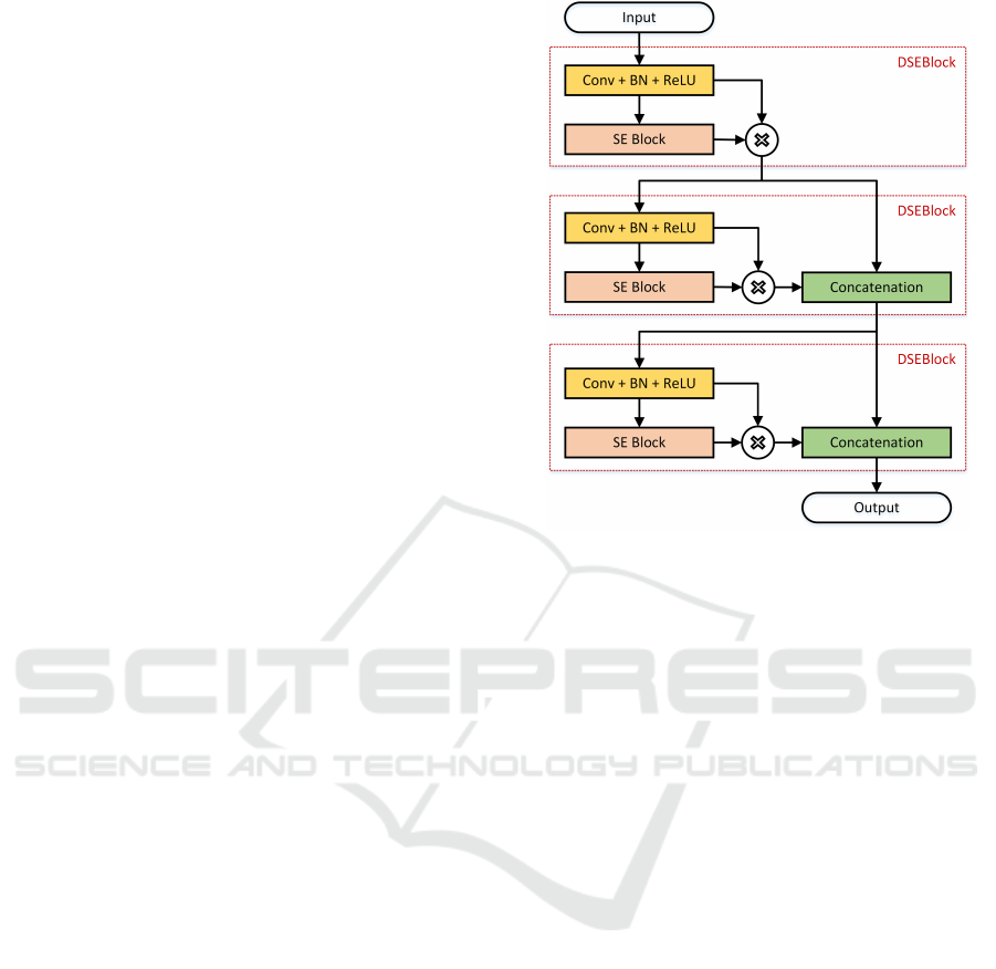
In all of them, we introduce the Dense Squeeze-
and-Excitation Block (DSEBlock) that is a combina-
tion of a DenseBlock (Huang et al., 2017) with the
Squeeze-and-Excitation (SE) mechanism (Hu et al.,
2018). The DenseBlock enhances the gradient flow
in the network and encourages feature reuse, while
Figure 2: Architecture of DSEBlock-3. DSEBlock-4 and
DSEBlock-5 are obtained by repeating the dashed block
once or twice more, respectively.
the SE re-weights the feature maps for better feature
learning. In a DSEBlock-n, the input is first fed to
a composite function consisting of a convolution fol-
lowed by a Batch Normalization (Ioffe and Szegedy,
2015) and then followed by a Rectified Linear Unit
(ReLU). The result is then passed to and also gated by
an SE block, whose architecture is described in (Hu
et al., 2018). This process is repeated n times with
skip connections to form a densely connected net-
work. For example, the architecture of DSEBlock-3
is shown in Figure 2.
4.1 Classification Net
By assuming that each segment of 2,000 I/Q samples
can contain at most one pulse, we design the Classi-
fication Net to classify a segment into one of the five
categories:
• ‘2 edges’: both TOA and TOD of a pulse appear
in the segment.
• ‘TOA only’: a TOA appears in the segment with-
out TOD.
• ‘TOD only’: a TOD appears in the segment with-
out TOA.
• ‘All pulse’: the whole segment is a part of a pulse.
• ‘All noise’: the segment contains only background
noise.
A Hierarchical Convolution Neural Network Scheme for Radar Pulse Detection
17
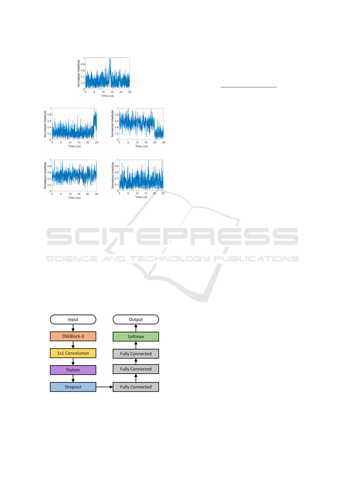
(a) 2 edges
(b) TOA only (c) TOD only
(d) All pulse (e) All noise
Figure 3: The 5 classes of segments of the signal envelop
for SNR = 6 dB at bandwidth 20 MHz.
Figure 3 depicts these classes under a relatively low–
SNR level.
The architecture of the Classification Net is shown
in Figure 4. This network consists of a DSEBlock-3
followed by a single filter of size 1 × 3, a Dropout
layer with dropping ratio of 0.5 and 4 fully connected
(FC) layers of size 128, 128, 128 and 5, respectively.
The first three FC layers use the ReLU activation
function, while the last FC layer is attached to a soft-
max function to output a score vector of length 5. In
each convolution layer of the DSEBlock-3, we use 16
filters of size 1 × 3.
Figure 4: Architecture of the Classification Net.
Each segment s of the signal ˆx
f
is treated as a 1-
D signal with two channels: channel-I (real part) and
channel-Q (imaginary part). Before feeding the seg-
ment to the Classification Net, we normalize it ac-
cording to:
s
norm
[n] =
s[n]
max
i
max{|s
I
[i]|, |s
Q
[i]|}
, ∀n. (3)
The cross-entropy loss function is used to train the
network. To decide the label of a segment, we in-
corporate the score vector output by the Classification
Net to an adaptive classification. This procedure takes
into account the following observations:(1) ‘2 edges’
cannot be followed by ‘All pulse’; (2) ‘TOA only’
cannot be followed by ‘All noise’; (3) ‘TOD only’
cannot be followed by ‘All pulse’; (4) ‘All pulse’ must
be followed by ‘TOD only’ or ‘All pulse’ and (5) ‘All
noise’ cannot be followed by ‘TOD only’ and ‘All
pulse’. Therefore, the main idea of the adaptive clas-
sification is that we exclude impossible labels from
the score vector of the current segment based on the
label of the previous one, if its confidence was high;
then take argument max of the rest as the label and its
score as the confidence of the current segment. This
is repeated until the end of the signal.
4.2 Denoising Net
We adopt a residual learning strategy (Zhang et al.,
2017) for the Denoising Net. The input of the network
is a noisy I/Q segment that includes a TOA and/or
a TOD and the output is a perturbation of the same
size that will be subtracted from the input to compen-
sate for the noise. The network is trained to minimize
the mean squared error between the output and the
ground-truth noise, which is a segment of w
f
given in
(2).
The architecture of the Denoising Net is sketched
in Figure 5. It incorporates DSEBlocks into an
encoder-decoder network with symmetric skip con-
nections (Mao et al., 2016) in the same spirit as (J
´
egou
et al., 2017). Here, we use five DSEBlock-5, each of
which is followed by a 1 × 1 convolution layer to re-
duce the number of feature maps by a factor of 5. In-
side a DSEBlock-5, the number of filters used in the 5
convolution layers are 32, 48, 64, 80 and 96, respec-
tively; all filters are of size 1 × 7. The Downsampling
is simply a 1 × 2 max pooling. The Upsampling is a
1 × 7 transposed convolution with stride 2.
4.3 Edge-detection Nets
To locate the edges in a segment, the magnitude of
the output of Denoising Net is passed to one of three
Edge–Detection Nets: TOA Net, TOD Net and TOA-
TOD Net. Which network is used depends on the re-
ICPRAM 2020 - 9th International Conference on Pattern Recognition Applications and Methods
18
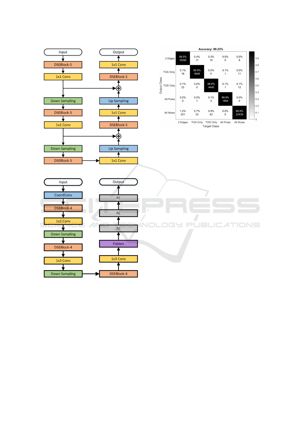
Figure 5: Architectures of the Denoising Net.
Figure 6: Architecture of the Edge Detection Nets (TOA
Net, TOD Net, and TOA-TOD Net). The output of TOA
Net or TOD Net is a scalar, whereas the output of TOA-
TOD Net is a two-dimension vector.
sult of the segment classification, as shown in Fig-
ure 1. These three networks share the same architec-
ture as depicted in Figure 6 but are trained separately
on different datasets. The Coordinate-Convolution
(CoordConv) layer (Liu et al., 2018) simply maps the
coordinates of all samples in the segment to an ar-
ray in [−1, 1] and then appends it to the input as a
new channel. This is to incorporate the location in-
formation into the learning for better edge detection.
The result is then passed to a concatenation of three
Figure 7: Confusion matrix of Classification Net on the test
set.
DSEBlock-4, each of which is followed by a 1 × 3
convolution layer that reduces the number of feature
maps by a factor of 4. The first two of them are fur-
ther attached to a Downsampling that is a 1 × 2 max
pooling. We use 16, 8 and 4 filters in each convolu-
tion layer of the first, second, and third DSEBlock-4,
respectively; all filters are of size 1 × 3.
The tail of the network is a concatenation of 3 FC
layers: the first two layers are of size 128 and the last
one is of size 1 (for TOA Net and TOD Net) or 2 (for
TOA-TOD Net). By using the sigmoid function in the
end, the outputs of edge-detection nets are always in
[0, 1]. Each network is trained to minimize the Mean
Absolute Error (MAE) between output and ground-
truth TOA and/or TOD, which are also normalized to
[0, 1].
5 PERFORMANCE EVALUATION
In this section, we provide some results for simulated
radar pulses. All data were generated by a simula-
tor written in Matlab. The training of proposed sub-
networks was implemented in Python with Keras li-
brary and TensorFlow backend running on 4 Nvidia
Tesla P100 GPUs. The training data for all networks
are segments of 2,000 I/Q samples, each of which is
randomly truncated from a longer signal that contains
a rectangular radar pulse. Each pulse was randomly
generated with one of the seven aforementioned mod-
ulation types, over a pulse width in [0.1, 400] µs and
with an SNR (over the 20 MHz bandwidth) in [0, 15]
dB. All sub-networks were trained for 100 epochs us-
ing an Adam optimizer with a learning rate of 10
−4
and the best models are selected for DeepIQ.
Firstly, the Classification Net was trained on
1,000,000 examples labeled with five categories: ‘2
A Hierarchical Convolution Neural Network Scheme for Radar Pulse Detection
19
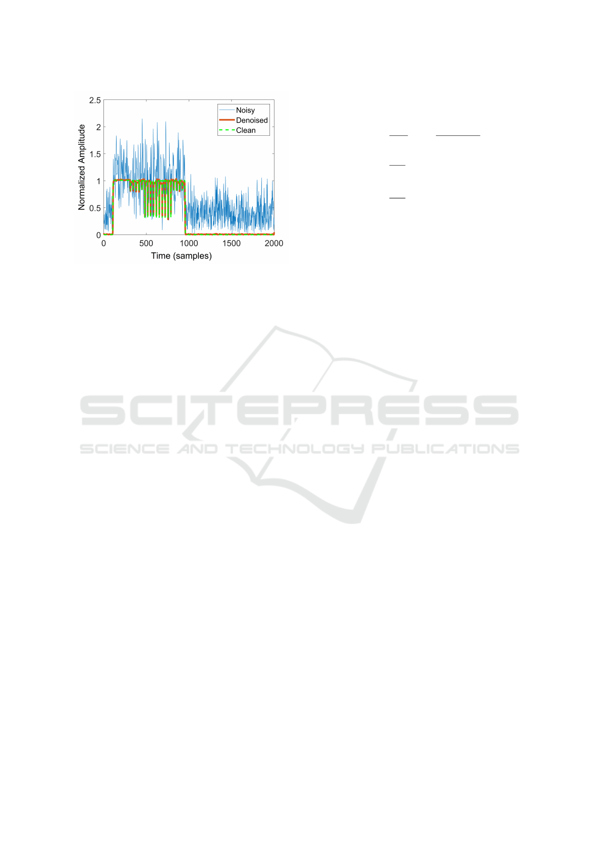
Figure 8: An example of denoising of a modulated radar
pulse.
edges’, ‘TOA only’, ‘TOD only’, ‘All pulse’ and ‘All
noise’. The best model was tested on another sepa-
rated set of 50,000 examples, yielding an overall ac-
curacy of 99.23% with the confusion matrix shown in
Figure 7. Secondly, the Denoising Net was trained on
500,000 segments of the first three labels. The result-
ing model was able to improve the average SNR of
150, 000 testing examples by 22.43 dB. Figure 8 vi-
sualizes the denoising of an example received noisy
radar pulse. Finally, the TOA Net, TOD Net and
TOA-TOD Net were trained on three different sets,
each of which includes the envelops of 500, 000 sam-
ples of denoised segments with labels ‘TOA only’,
‘TOD only’ and ‘2 edges’, respectively. These net-
works achieved the MAEs of 26.38 ns, 26.45 ns and
27.67 ns on average, respectively, over separated test
sets of 150,000 samples each. To test the whole detec-
tion procedure, we run DeepIQ scheme on segments
of a long signal containing N
true
= 10, 000 pulses
equally separated by 6, 000 samples under different
SNR levels. Two pulses output by DeepIQ are merged
into one if the distance between them is less than 25
µs. Then, we evaluate the performance of the pro-
posed DeepIQ network in both detection and estima-
tion metrics.
Let us denote the list of ground-truth TOAs and
TODs by {(a
i
, d
i
)}
N
true
i=1
and the list of estimated TOAs
and TODs by {( ˆa
i
,
ˆ
d
i
)}
N
est
i=1
. A pulse (a
i
, d
i
) is called
detected if there exists j ∈ {1, 2, . . . , N
est
} such that:
|a
i
− ˆa
j
| < 200 ns. (4)
By renumbering, assuming that the detected pulses
{(a
i
, d
i
)}
N
det
i=1
are matched by the subset {( ˆa
i
,
ˆ
d
i
)}
N
det
i=1
of estimated pulses. The remaining pulses,
{( ˆa
i
,
ˆ
d
i
)}
N
est
i=N
det
+1
, are considered false alarms. The
detection performance is then measured by the fol-
lowing four metrics: the detection rate, the F1 score,
the TOA Mean Absolute Error (MAE) and and the
TOD MAE, which are computed as:
P
d
=
N
det
N
true
, F
1
=
2N
det
N
true
+ N
est
,
∆
TOA
=
1
N
det
N
det
∑
i=1
|a
i
− ˆa
i
|,
∆
TOD
=
1
N
det
N
det
∑
i=1
|d
i
−
ˆ
d
i
|.
Note that the detection rate measures the sensitivity
of the algorithm while the F1 score balances the true
detection rate and the false alarm rate.
To evaluate the performance of our proposed
scheme in this paper, we compare the detection accu-
racy of DeepIQ with that of the Threshold-based Edge
Detection (TED) algorithm (Iglesias et al., 2014) and
our previous work based on Find–Change–Points al-
gorithms (FCA) (Nguyen et al., 2019). Table 1 reports
the detection performances of three methods for vari-
ous SNR levels from 0 dB to 15 dB. It can be seen that
DeepIQ achieves the superior performance compared
with TED and FCA in all measures and for all SNR
levels. Especially, the performance gaps are strikingly
much larger in low-SNR regimes. For example, in the
extremely noisy case when SNR = 0 dB, the proposed
scheme DeepIQ is able to boost the F1 score from
1.59% of TED and 32.72% of FCA to 55.57%. Fur-
thermore, DeepIQ achieves a reduction of 38 ns and
22 ns in the TOA MAE as compared with TED and
FCA. The TOD MAE of DeepIQ is also 27.15 and
6.74 times smaller than that of TED and FCA, respec-
tively.
Our proposed scheme DeepIQ is a better solution
to solve the radar pulse detection compared with pre-
vious schemes because of the following underlying
reasons:
• Firstly, noise floor estimation is a prerequisite in
previous TED schemes in order to determine de-
tection threshold. However, in low–SNR levels,
accuracy estimation of detection threshold is a
very difficult task due to the effect of noise. Im-
proper detection threshold leads to a significant
degradation of radar pulse detection, for e.g. high
false alarm and missed detection rates. Thanks
to the proposed classification neural network with
deep-learning approach which reduces the tedious
detection threshold setting, DeepIQ reaches a bet-
ter detection if a radar pulse is present, partially
present of absent in the received signal.
• Secondly, previous methods including our pre-
vious work apply traditional algorithms such as
threshold based algorithm (TED) or find-change-
point algorithm (FCA) to estimate the TOA and
ICPRAM 2020 - 9th International Conference on Pattern Recognition Applications and Methods
20
Table 1: Performance comparison of schemes with different
SNR levels at the bandwidth of 20 MHz.
TOD positions in the edges of radar pulse. The
drawback of these approaches is the edges of radar
pulse are deformed critically under the effect of
noise in low–SNR levels. Therefore, it is very dif-
ficult to estimate correctly in such conditions. By
applying the state-of-the art techniques in the pro-
posed Denoising Net and Edge–Detection Nets,
DeepIQ can mitigate the effect of noise as well
as achieve a significant improvement of detection
accuracy in severe conditions.
6 CONCLUSION
In this paper, we have introduced a hierarchical con-
volution neural network scheme, DeepIQ, for the de-
tection of radar pulses with various waveforms over
a wide range of SNR levels. The proposed scheme
is obtained by assembling 5 sub-convolution neural
network that are in charge of 3 different roles: clas-
sification, denoising, and edge detection. These net-
works are trained on radar I/Q segments of a fixed
length. The simulation results show that DeepIQ sig-
nificantly outperforms the Threshold-based Edge De-
tection (TED) scheme (Iglesias et al., 2014) and our
previous work (Nguyen et al., 2019) especially for
low SNR levels. The shortcoming of our method is
its computation time, about 0.44 µs/sample on one
GPU, which is still far from the real-time target,
12.8 ns/sample. Future work should focus on com-
pressing DeepIQ’s sub-networks as suggested in (Han
et al., 2016).
REFERENCES
Albaker, B. M. and Rahim, N. A. (2011). Detection and pa-
rameters interception of a radar pulse signal based on
interrupt driven algorithm. Int. Conf. on Emerging Re-
search in Computing, Information, Communications
and Applications (ERCICA), 6:1380–1387.
Goodfellow, I., Bengio, Y., and Courville, A. (2016). Deep
Learning. MIT Press.
Han, S., Mao, H., and Dally, W. J. (May 02-04, 2016).
Deep compression: Compressing deep neural net-
works with pruning, trained quantization and huffman
coding. In Proc. Int. Conf. Learning Representations
(ICLR), pages 1–14, Puerto Rico.
He, K., Zhang, X., Ren, S., and Sun, J. (Jun. 27-30, 2016).
Deep residual learning for image recognition. In Proc.
Conf. Comput. Vis. Pattern Recogn. (CVPR), pages
770–778, Las Vegas, NV, USA.
Hu, J., Shen, L., and Sun, . (June 18-22, 2018). Squeeze-
and-Excitation networks. In Proc. Conf. Comput. Vis.
Pattern Recogn. (CVPR), pages 7132–7141, Salt Lake
City, UT, USA.
Huang, G., Liu, Z., van der Maaten, L., and Weinberger,
K. Q. (July 21-26, 2017). Densely connected convo-
lutional networks. In Proc. Conf. Comput. Vis. Pat-
tern Recogn. (CVPR), pages 4700–4708, Honolulu,
HI, USA.
Iglesias, V., Grajal, J., Yeste-Ojeda, O., Garrido, M.,
S
´
anchez, M. A., and L
´
opez-Vallejo, M. (May 19-23,
2014). Real-time radar pulse parameter extractor. In
Proc. IEEE Radar Conf., pages 1–5.
Ioffe, S. and Szegedy, C. (Jul. 06-11, 2015). Batch nor-
malization: Accelerating deep network training by re-
ducing internal covariate shift. In Proc. Int. Conf.
Machine Learning (ICML), pages 1097–1105, Lille,
France.
J
´
egou, S., Drozdzal, M., Vazquez, D., Romero, A., and Ben-
gio, Y. (2017). The one hundred layers tiramisu: Fully
convolutional DenseNets for semantic segmentation.
arXiv:1611.09326 [cs.CV].
Killick, R., Fearnhead, P., and Eckley, I. A. (2012). Optimal
detection of changepoints with linear computational
cost. J. Am. Stat. Assoc., 107(500):1590–1598.
Krizhevsky, A., Sutskever, I., and Hinton, G. E. (Dec. 03-
08, 2012). Imagenet classification with deep convo-
lutional neural networks. In Proc. Adv. Neural Inf.
Process. Syst. (NIPS), pages 1097–1105, Lake Tahoe,
NV, USA.
Lakshmi, G., Gopalakrishnan, R., and Kounte, M. R.
(2013). Detection and extraction of radio frequency
and pulse parameters in radar warning receivers. In
Scientific Research and Essays, pages 632–638.
A Hierarchical Convolution Neural Network Scheme for Radar Pulse Detection
21

Lancon, F., Hillion, A., and Saoudi, S. (1996). Radar sig-
nal extraction using correlation. In European Signal
Processing Conf. (EUSIPCO), pages 632–638.
LeCun, Y., Bengio, Y., and Hinton, G. (2015). Deep learn-
ing. Nature, 521:436–444.
Levanon, N. and Mozeson, E. (2004). Radar Signals.
Wiley-Interscience.
Liu, R., Lehman, J., Molino, P., and Such, F. P. (2018).
An intriguing failing of convolutional neural net-
works and the CoordConv solution. arXiv:1807.03247
[cs.CV].
Liu, W., Anguelov, D., Erhan, D., Szegedy, C., Reed, S.,
Fu, C.-Y., and Berg, A. C. (Oct. 08-16, 2016). SSD:
Single shot multibox detector. In Proc. Eur. Conf.
Comput. Vis. (ECCV), pages 21–37, Amsterdam, The
Netherlands.
Mao, X.-J., Shen, C., and Yang, Y.-B. (Dec. 05-10,
2016). Image restoration using very deep convolu-
tional encoder-decoder networks with symmetric skip
connections. In Proc. Adv. Neural Inf. Process. Syst.
(NIPS), pages 1–9, Barcelona, Spain.
Nguyen, H. Q., Ngo, D. T., and Do, V. L. (2019). Deep
learning for radar pulse detection. In Int. Conf.
on Pattern Recognition Applications and Methods
(ICPRAM), pages 32–39.
Pace, P. E. (2009). Detecting and Classifying Low Proba-
bility of Intercept Radar. Artech House, 2 edition.
Poisel, R. (2005). EW Target Location Methods. Artech
House.
Redmon, J., Divvala, S., Girshick, R., and Farhadi, A. (Jun.
27-30, 2016). You Only Look Once: Unified, real-
time object detection. In Proc. Conf. Comput. Vis. Pat-
tern Recogn. (CVPR), pages 779–788, Las Vegas, NV,
USA.
Ren, S., He, K., Girshick, R., and Sun, J. (2017). Faster
R-CNN: Towards real-time object detection with re-
gion proposal networks. IEEE Trans. Pattern Anal.
Machine Intell., 39(6):1137–1149.
Richards, M. A. (2014). Fundamental of Radar Signal Pro-
cessing. McGraw-Hill Education, 2 edition.
Szegedy, C., Liu, W., Jia, Y., Sermanet, P., Reed, S.,
Anguelov, D., Erhan, D., Vanhoucke, V., and Rabi-
novich, A. (Jun. 07-12, 2015). Going deeper with
convolutions. In Proc. Conf. Comput. Vis. Pattern
Recogn. (CVPR), pages 1–9, Boston, MA, USA.
Torrieri, D. J. (1974). Arrival time estimation by adaptive
thresholding. IEEE Trans. Aerospace Electro. Sys-
tems, AES-10(2):178–184.
Torrieri, D. J. (1984). Statistical theory of passive location
systems. IEEE Trans. Aerospace Electro. Systems,
AES-20(2):183–198.
Zhang, K., Zuo, W., Chen, Y., Meng, D., and Zhang, L.
(2017). Beyond a Gaussian denoiser: Residual learn-
ing of deep CNN for image denoising. IEEE Trans.
Image Process., 26(7):3142–3155.
ICPRAM 2020 - 9th International Conference on Pattern Recognition Applications and Methods
22
