3DSAL: An Efﬁcient 3D-CNN Architecture for Video Saliency Prediction

Yasser Abdelaziz Dahou Djilali

1,3

, Mohamed Sayah

, Kevin McGuinness

and Noel E. O’Connor

Institut National des T

ecommunications et des TIC, Oran, Algeria

Universit

e Oran1, FSEA, Oran, Algeria

Insight Center for Data Analytics, Dublin City University, Dublin 9, Ireland

Keywords:

Visual Attention, Video Saliency, Deep Learning, 3D CNN.

Abstract:

In this paper, we propose a novel 3D CNN architecture that enables us to train an effective video saliency

prediction model. The model is designed to capture important motion information using multiple adjacent

frames. Our model performs a cubic convolution on a set of consecutive frames to extract spatio-temporal

features. This enables us to predict the saliency map for any given frame using past frames. We comprehensively

investigate the performance of our model with respect to state-of-the-art video saliency models. Experimental

results on three large-scale datasets, DHF1K, UCF-SPORTS and DAVIS, demonstrate the competitiveness of

our approach.

1 INTRODUCTION

Human attention was considered ﬁrst in philosophy,

later in psychology and neuroscience, and most re-

cently as a computer vision problem in the ﬁeld of com-

puter science (Mancas et al., 2016). Thanks mainly to

advances in deep learning, the development of com-

putational models of human attention has received re-

newed research interest in recent years (Mancas et al.,

2016). Computational models have been proposed for

imitating the attentional mechanisms of the Human

Visual Systems (HVS) for both dynamic and static

scenes. Dynamic ﬁxation prediction, or video saliency

prediction, is very useful for understanding human at-

tentional behaviors for video content and has multiple

practical real-world applications e.g. video captioning,

compression, question answering, and object segmen-

tation (Wang et al., 2018). It is thus highly desirable

to have robust high-performance video saliency pre-

diction models.

Recently introduced benchmarks, such as

DHF1K (Wang et al., 2018) and LEDOV (Jiang

et al., 2018a), have allowed researchers to effectively

train deep learning models in an end-to-end manner

by formulating saliency as a regression problem.

However, the reported performances on video

(dynamic scene) datasets according to commonly used

saliency metrics are still far from those reported for

images (static scene). This is most likely due to the

rapid transition of video frames that makes dynamic

saliency prediction very challenging. Latent video

saliency deep learning based models separate spatial

features from temporal features. This is implemented,

for example, by a CNN module to extract spatial

features, which can then be aggregated into an LSTM

module to capture the temporal features (Hochreiter

and Schmidhuber, 1997).

In this paper we propose a novel video saliency

model that uses a 3D CNN architecture (Ji et al., 2013).

When performing a cubic convolution, our model cap-

tures spatio-temporal features in one 3D CNN module.

The dimensions

and

of the cube extract the spatial

features while the

axis extracts the temporal features.

In this way, the model learns saliency by fusing spatio-

temporal features for calculating the ﬁnal saliency map.

Our key contribution is a 3D CNN architecture for pre-

dicting human gaze in dynamic scenes, which explic-

itly learns the hidden relationship between adjacent

frames for accurate saliency prediction.

This paper is organized as follows: Section

2 provides an overview of related video saliency

works. Section 3 gives a detailed description of

the proposed deep saliency framework. Section 4

compares the experimental results to state-of-the-art

methods. Finally, we conclude this work in Sec-

tion 5. The results can be reproduced with the

source code and trained models available on GitHub:

https://github.com/YasserDA/Saliency-3DSal.

Djilali, Y., Sayah, M., McGuinness, K. and O’Connor, N.

3DSAL: An Efﬁcient 3D-CNN Architecture for Video Saliency Prediction.

DOI: 10.5220/0008875600270036

In Proceedings of the 15th International Joint Conference on Computer Vision, Imaging and Computer Graphics Theory and Applications (VISIGRAPP 2020) - Volume 4: VISAPP, pages

27-36

ISBN: 978-989-758-402-2; ISSN: 2184-4321

2 RELATED WORK

In this section we review the relevant literature on

saliency models for both static and dynamic scenes.

2.1 Static Saliency Models

Saliency prediction for images has been widely studied

during the last few decades. As a pioneer, (Itti et al.,

1998) derived bottom-up visual saliency using center-

surround differences across multi-scale image features.

Other static saliency models e.g. (Bruce and Tsot-

sos, 2006; Garcia-Diaz et al., 2009; Seo and Milanfar,

2009; Goferman et al., 2012; Gao and Vasconcelos,

2005) are mostly based on computing multiple visual

features such as color, edge, and orientation at mul-

tiple spatial scales to produce a saliency map. More

recent deep learning based static saliency models e.g.

(Huang et al., 2015; K

ummerer et al., 2014; Liu et al.,

2015; Kruthiventi et al., 2017; Cornia et al., 2016; Pan

et al., 2016; Pan et al., 2017) have achieved remark-

able improvements relying on the success of neural

networks and the availability of large-scale saliency

datasets for static scenes, such as those described in

(Bylinskii et al., ; Jiang et al., 2015; Borji and Itti,

2015).

(Vig et al., 2014) and (Kruthiventi et al., 2017)

were the ﬁrst to use CNNs for saliency prediction when

introducing eDN and DeepFix respectively. DeepFix

initialized the ﬁrst 5 convolution blocks with VGG-16

weights, then added two novel Location Based Convo-

lutional (LBC) layers to capture semantics at multiple

scales. Pan et al. (Pan et al., 2017) used Generative Ad-

versarial Networks (GANs) (Goodfellow et al., 2014)

to build the SalGAN model. The network consists

of a generator model whose weights are learned by

back-propagation computed from a binary cross en-

tropy (BCE) loss over existing saliency maps. The

resulting prediction is processed by a discriminator

network trained to solve a binary classiﬁcation task

between the saliency maps generated by the generative

stage and the ground truth ones.

2.2 Dynamic Saliency Models

Visual information constantly changes due to egocen-

tric movements or the dynamics of the scene being

observed. Dynamic saliency is then dependent on

both current scene saliency as well as the accumulated

knowledge from previous time instants (Borji and Itti,

2013). Video saliency prediction is extremely more

challenging than image saliency prediction (Borji,

2018). In this task, viewers have much less time to

explore each video frame (

∼ 1/30

seconds) compared

to the 3-5 seconds typical for viewing still images.

Early video saliency models such as (Leifman

et al., 2017; Garcia-Diaz et al., 2012; Zhang and

Sclaroff, 2013; Leboran et al., 2017; Xu et al., 2017;

Guo et al., 2008; Rudoy et al., 2013), rely on existing

static saliency models with additional motion features.

They generally use linear or nonlinear combination

rules to fuse spatial and temporal information. How-

ever, using a simple ﬁxed weight to combine spatial

and temporal information can drive the model to lose

the intrinsic relationship between these two comple-

mentary aspects.

A few works have investigated deep learning based

video saliency prediction models (Bak et al., 2018;

Jiang et al., 2017; Wang et al., 2018; Adel Bargal et al.,

2018). These are mainly based on two distinct net-

work modules to deal with spatial and temporal ﬁelds

separately. These works exhibit strong performance

and show the potential of using neural networks to the

video saliency problem. (Bak et al., 2018) were the

ﬁrst to leverage deep learning when they used a two-

stream CNN architecture for video saliency prediction.

Video frames and motion maps were fed to the two

streams. (Wang et al., 2018) proposed a CNN-LSTM

network architecture with an attention mechanism to

explicitly encode static saliency information, thus al-

lowing the LSTM to focus on learning a more ﬂexi-

ble temporal saliency representation across successive

frames. (Linardos et al., 2018) introduced a temporal

regularization for their previous model SalGAN (Pan

et al., 2017) for static saliency prediction. In terms of

architecture, they added a convolutional LSTM layer

on top of the frame-based saliency prediction to adapt

it for dynamic saliency prediction.

All these works consider the spatial domain as the

most inﬂuential aspect, and use very little accumulated

knowledge from the past (

∼ 70ms

), while the aver-

age human eye reaction time, is of the order of

284ms

(Saslow, 1967). We propose that more importance

needs to be given to the temporal domain for video

saliency prediction. In our approach, we exploit the

temporal and spatial domain in an equal manner via

the use of 3D CNN, with a view to more appropriate

spatio-temporal feature learning (see Fig. 1). Further-

more, we smooth adjacent frames to obtain good eye

ﬁxation quality saturation by introducing the tangent

hyperbolic weighting function on the input sequence

frames.

VISAPP 2020 - 15th International Conference on Computer Vision Theory and Applications

3 OUR APPROACH

3.1 Overview

Fig. 2 represents the overall architecture of our video

saliency model. The framework takes

consecu-

tive input frames:

t−i

∈ R

224×244×3

: i ∈ {0,...,5}}

Since the latency for saccadic eye movement is about

284

ms (Saslow, 1967), when watching a 30 fps video,

the human eye is sensitive to exactly

(0.284ms × 30

fps)

' 8

frames. Thus, we set the number of input

frames to six to approximate the ideal threshold and

save computing capacity at the same time. Each frame

is fed into the spatial feature extraction function mod-

eled with a pre-trained VGG-16 (Simonyan and Zis-

serman, 2014) after removing the fully connected lay-

ers. This choice was motivated by the reduction of

complexity while improving accuracy. Since VGG-16

was trained on large-scale ImageNet dataset (1.4M im-

ages) (Deng et al., 2009), VGG-16 provides excellent

feature extraction performance. The output of the spa-

tial feature extraction function is six feature cuboids:

∗

t−5

∗

t−4

,.....,F

∗

∈ R

14×14×512

, with

G(F

) = F

∗

, (1)

and where the function

is modelled by the truncated

VGG-16 model (for more details see (Simonyan and

Zisserman, 2014)).

3.2 Weighting Cuboid Coefﬁcients

The eye motion on a given object has been intuitively

considered as a tangent hyperbolic activation func-

tion (Nwankpa et al., 2018). To preserve the consis-

tency of human vision and avoid computing complex-

ity in time and space, we considered six frames to

deﬁne the motion features for the human eyes. This

enables us to use a suitable

tanh

function, to weight the

motion frames by parameters

c[i]

where

i ∈ {1,..., 6}

–

see bold weights in Table 1.

Considering the vector of parameters

c =

[0.4,0.5,0.6, 0.7,0.8,0.98]

as illustrated in Table 1, we

can reach the eye ﬁxation quality saturation in the 6

spatial frame. As such, the temporal dimension is

Figure 1: 3D Convolution operation over adjacent frames.

Table 1: Fixation quality motion.

Weight Fixation Quality Quality

Quality Variation Saturation

c[i] tanh(c[i]) tanh(c[i+1]) tanh(c[i+1])

−tanh(c[i]) +tanh(c[i])

0.1 0,044 - -

0.2 0,088 0.044 0.13

0.3 0,134 0.046 0.22

0.4 0.184 0.050 0.32

0.5 0.239 0.055 0.42

0.6 0.301 0.062 0.54

0.7 0.377 0.076 0.68

0.8 0.477 0.100 0.85

0.98 0.998 0.521 1.47

- 0,998 0,0 2.00

deﬁned as a continuation of six

-weighted consecu-

tive frames. In each iteration, the

spatial frame

is determined via an adversarial process in which the

spatial frames

t−5

t−4

t−3

t−2

, and

t−1

are used

to compute the

saliency map. Finally, each of the six

cuboids, weighted with respect to their importance in

the learning process, are adjusted in a temporary order

to construct one spatio-temporal feature map. Note

that the six frames do not represent a large variation of

space and that their concatenation preserves the spa-

tial information when ﬁnding the correlation in time

for each pixel location. Later, a spatio-temporal fea-

ture map of

6×

frames determines the spatio-temporal

units

S ∈ R

6×14×14×512

. The 3D CNN takes

as an

input, to perform a spatio-temporal fusion, in order to

learn saliency. Then, a saliency map

P ∈ R

224×224

generated to represent the saliency map for F

3.3 3D CNN Architecture

We believe that a 3D ConvNet is more appropriate for

spatio-temporal feature learning. Compared to a 2D

ConvNet, a 3D ConvNet has the ability to model tem-

poral information better by virtue of 3D convolutions

and 3D pooling operations. In 2D ConvNets, convo-

lution and pooling operations are only performed spa-

tially. 3D ConvNets perform those operations spatio-

temporally to preserve temporal information in the

input signals resulting in an output volume (see Fig. 1).

The same phenomena is applicable for 2D and 3D

pooling (Tran et al., 2015).

As shown in Table 2, we built a ﬁve block decoder

3D CNN network to learn saliency in a

slow f usion

manner. Each block consists of Deconv3D and opera-

tions, with a ReLU (Rectiﬁed Linear Unit) activation

function. The role of Deconv3D is to up-sample the

feature map resolution and Conv3D to construct the

3DSAL: An Efﬁcient 3D-CNN Architecture for Video Saliency Prediction

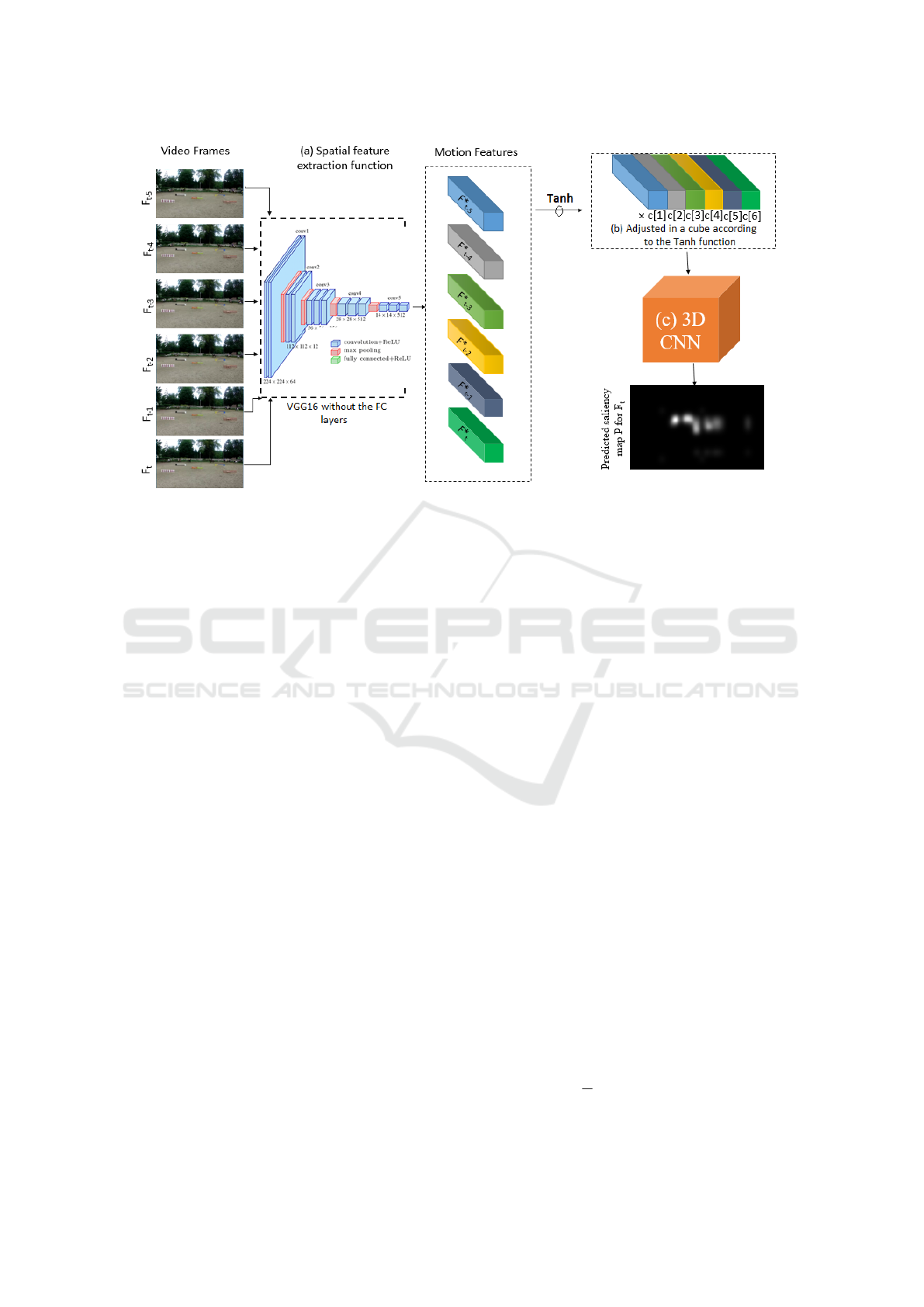
Figure 2: Network Architecture of 3DSAL. (a) Feature extraction function with the truncated VGG-16. (b) Composition of

adjacent feature maps via the use of Tanh activation function. (c) Spatio-temporal feature fusion with 3D CNN.

spatio-temporal features for saliency learning. We de-

note the triplet

(t,r,s)

as the kernel size for Deconv3D

and Conv3D layers. We use the

axis in the kernel

to cover the temporal dimension in the kernel, while,

(r, s)

denotes the spatial kernel size. Consider a convo-

lutional layer

and the input spatio-temporal units

The

output unit

i,K

(l)

for the layer

is computed

as:

(l)

i,K

(x,y,z)

∑

c=1

∑

t=1

∑

r=1

∑

s=1



(l)

i,K,c

(t,r,s)

× U

(l−1)

i,c

(x+t,y+r,z+s)



(l)

i,K

(2)

where

is the channel number for the layer

(l)

and

x,y, z

are the cubic spatial dimensions. The parame-

ter

is considered as the channel dimension for the

output unit

(l)

. The

(l)

i,K,c

term denotes the weights

connecting the

unit at position

(x,y, z)

in the feature

map of layer

(l − 1)

and the

unit in the layer

with

channels. Finally, the

(l)

∀i,K

term is the bias vector

with length K.

The authors of (Li et al., 2016) and (Tran et al.,

2015) demonstrated that the most suitable kernel size

for 3D convolution is

3 × 3 × 3

. Hence, we set the

3D convolution kernel size to

3 × 3 × 3

with stride

1 × 1 × 1

. Since the ground truth saliency map can

be seen as a distribution probability, where each pixel

represents the probability to be ﬁxated by a human, at

the ﬁnal block, we use the sigmoid as an activation

function to get a normalized predicted saliency map in



0,1] with a size 224 ×224.

Loss function

. The saliency loss is computed on

a per-pixel basis, where each value of the predicted

saliency map is compared with its corresponding peer

from the ground truth map. We denote the predicted

saliency map as

P ∈



0,1]

224×224

and the continuous

saliency map as

G ∈



0,1]

224×224

. The continuous

saliency map

is obtained by blurring the binary ﬁxa-

tion map

with a 2D Gaussian kernel. The ﬁxation

map FM is a binary image with:

i j

(

1 if location (i, j ) is a ﬁxation

0 otherwise,

and the variance of the Gaussian is selected so the

ﬁlter covers approximately 1-degree of visual angle,

as done in (Judd et al., 2012). The saliency task can be

seen as a similarity measure between the predicted

saliency map

and the ground truth

. The loss

function must be designed to maximise the invariance

of predictive maps and give higher weights to locations

with higher ﬁxation probability. An appropriate loss

for this situation is the binary cross entropy, deﬁned

as:

BCE

(G,P) = −

∑

i=1

log(P

) + (1 − G

)log(1 − P

))

(3)

VISAPP 2020 - 15th International Conference on Computer Vision Theory and Applications

Table 2: Architecture of the 3D CNN.

Layer Depth Kernel Output Params Act

/Pool Shape #

Conv3D 1 1 512 3 × 3 × 3 (6,14,14,512) 7078400 ReLU

Conv3D 1 2 512 3 × 3 × 3 (6,14,14,512) 7078400 ReLU

MaxPool3D 1 – 4 × 2 × 2 (3,7,7,512) 0 –

Batch-Norm – – (3,7,7,512) 2048 –

Deconv3D 1 512 1 × 3 × 3 (3,14,14,512) 2359808 ReLU

Conv3D 2 1 512 3 × 3 × 3 (3,14,14,512) 7078400 ReLU

Batch-Norm – – (3,7,7,512) 2048 –

Deconv3D 2 256 3 × 3 × 3 (3,28,28,256) 3539200 ReLU

Conv3D 2 1 256 3 × 3 × 3 (3,28,28,256) 179728 ReLU

Conv3D 2 2 256 3 × 3 × 3 (3,28,28,256) 179728 ReLU

MaxPool3D 2 – 3 × 1 × 1 (1,28,28,256) 0 –

Batch-Norm – – (1,28,28,256) 1024 –

Deconv3D 3 128 1 × 3 × 3 (1,56,56,128) 295040 ReLU

Conv3D 3 1 128 1 × 3 × 3 (1,56,56,128) 147584 ReLU

Conv3D 3 2 128 1 × 3 × 3 (1,56,56,128) 147584 ReLU

Batch-Norm – – (1,56,56,128) 512 –

Deconv3D 4 64 1 × 3 × 3 (1,112,112,64) 73792 ReLU

Conv3D 4 1 64 1× 3 × 3 (1,112,112,64) 36928 ReLU

Conv3D 4 2 64 1× 3 × 3 (1,112,112,64) 36928 ReLU

Batch-Norm – – (1,112,112,64) 2048 –

Deconv3D 5 32 1 × 3 × 3 (1,224,224,32) 18464 ReLU

Conv3D 5 1 32 1× 3 × 3 (1,224,224,32) 9258 ReLU

Conv3D 5 2 16 1× 3 × 3 (1,224,224,16) 4624 ReLU

Conv3D 5 3 1 1 × 3 × 3 (1,224,224,1) 145 Sigm

Total Params: 31,447,841

4 EXPERIMENTS

4.1 Experimental Setup

Datasets

. DHF1K (Wang et al., 2018), LEDOV (Jiang

et al., 2018b), HOLYWOOD (Mathe and Sminchis-

escu, 2015), UFC-SPORT (Mathe and Sminchis-

escu, 2015) and DIEM (Mital et al., 2011) are the

ﬁve datasets widely used for video saliency research.

DHF1K comprises a total of 1,000 video sequences

with 582,605 frames covering a wide range of scenes,

motions and activities. HOLLYWOOD-2 is a dynamic

eye tracking dataset. It contains short video sequences

from a set of 69 Hollywood movies, containing 12 dif-

ferent human action classes, ranging from answering

a phone, eating, driving and running. The UCF-Sports

dataset consists of 150 videos covering 9 sports classes

like golf, skateboarding, running and riding. LEDOV

contains videos with a total of 179,336 frames cover-

ing three main sub-categories: Animals, Man-made-

Objects and Human activities varying from social ac-

tivities, daily actions, sports and art performance.

We have chosen DHF1K and UFC-SPORT to train

our 3DSAL model. DHF1K characterises the free

viewing approach, in which subjects freely watch the

stimuli so that many internal cognitive tasks are en-

gaged, thereby making the generated saliency map

more difﬁcult to predict. UFC-SPORT is a task driven

dataset, where subjects are more likely to follow the

main objects in the scene, affording the model preci-

sion. Training on two different paradigms helps ensure

more robust prediction.

Training Protocol.

We have two training modes:

(1) 3DSAL-base: Training the model without regres-

sion, where all frames are fed into the 3D CNN in an

equal manner, without multiplying by the weighting

coefﬁcients. (2) 3DSAL-weighted: The use of weight-

ing coefﬁcients, to indicate the frame importance in

the prediction process.

For DHF1K, we respect the original train-

ing/validation/testing partitioning (600/100/300). For

UFC-SPORT, as proposed by the authors in (Mathe

and Sminchisescu, 2015), the training/testing is split

(103/47). We test our model on: DHF1K, UFC-

SPORT and DAVIS (Perazzi et al., 2016) for both

quantitative and qualitative results.

Technical Speciﬁcation.

We implemented our

model in Python using the Keras API running a Ten-

sorFlow backend. Due to the huge size of the train-

ing data (550k frames), we used the early stopping

technique on the validation set for optimal generaliza-

tion performance (Prechelt, 1998). The Adam Opti-

mizer (Kingma and Ba, 2014) initial learning rate was

set to

−4

and was dropped by 10 each 2 epochs. The

network was trained for 33 epochs. The entire training

procedure took about 7 days (160 hours) on a single

NVIDIA GTX 1080 GPU,which has a total of 8GB

global memory and 20 multiprocessors, and i7 7820

HK 3.9GHZ Intel processor.

Metrics.

To test the performance of our model,

we utilize the ﬁve widely used metrics: AUC-Judd

(AUC-J), Similarity metric (SIM), Linear Correlation

Coefﬁcient (CC), shufﬂed AUC (s-AUC) and Normal-

ized Scanpath Saliency (NSS). A detailed description

of these metrics is presented in (Borji and Itti, 2013).

Competitors.

We compare the performance of our

model according to the different saliency metrics, with

six video saliency models: OM-CNN (Jiang et al.,

2017), Two-stream (Bak et al., 2018), AWS-D (Lebo-

ran et al., 2017), OBDL (Hossein Khatoonabadi et al.,

2015), ACLNet (Wang et al., 2018), (Linardos et al.,

2018). Beneﬁting from the work of (Wang et al., 2018),

which tested the performance of the previous mod-

els in three datasets (DHF1K, HOLYWOOD-2, UFC-

SPORT), we add our results to this work, to compare

the performance of our model with these works.

4.2 Results

Table 3 shows the comparative study with the afore-

mentioned models according to the different saliency

metrics on DHF1K and UFC-SPORT datasets (300/47)

test videos. Our model is very competitive in the two

3DSAL: An Efﬁcient 3D-CNN Architecture for Video Saliency Prediction

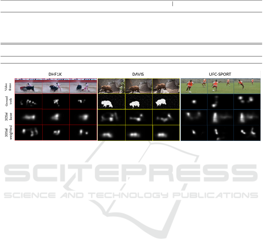
Table 3: Comparative performance study on: DHF1K, UFC-SPORT datasets.

Dataset DHF1K UFC-SPORT

AUC-J ↑ SIM ↑ s-AUC ↑ CC ↑ NSS ↑ AUC-J ↑ SIM ↑ s-AUC ↑ CC ↑ NSS ↑

# OBDL (Hossein Khatoonabadi et al., 2015) 0.638 0.171 0.500 0.117 0.495 0.759 0.193 0.634 0.234 1.382

# AWS-D (Leboran et al., 2017) 0.703 0.157 0.513 0.174 0.940 0.823 0.228 0.750 0.306 1.631

OM-CNN (Jiang et al., 2017) 0.856 0.256 0.583 0.344 1.911 0.870 0.321 0.691 0.405 2.089

Two-Stream (Bak et al., 2018) 0.834 0.197 0.581 0.325 1.632 0.832 0.264 0.685 0.343 1.753

ACLNET (Wang et al., 2018) 0.890 0.315 0.601 0.434 2.354 0.897 0.406 0.744 0.510 2.567

Linardos et al (Linardos et al., 2018) 0.744 0.260 0.722 0.302 2.246 – – – – –

3DSAL-Base – – – – – 0.8111 0.3255 0.6088 0.3209 1.7119

3DSAL-Weighted 0.8500 0.3205 0.6234 0.3562 1.9962 0.8813 0.4783 0.7011 0.5902 2.8023

(#) Non deep learning models. The best score is marked in bold red. The second best score is marked in bold black.

Figure 3: Saliency map predictions over three datasets.

datasets. The 3DSAL-weighted repeatedly appears

in the best two scores, and exhibits the best score

for certain metrics. Also, it is clear that deep learn-

ing approaches outperform classic hand-crafted video

saliency methods.

DHF1K.

The diversity of this dataset makes the

prediction task very challenging, our model remains

very competitive since our scores are close to the state

of art model (ACLNet (Wang et al., 2018)). This is

due to the inclusion of temporal domain exploration

via the use 3D CNN for adjacent frames.

UFC-SPORT.

On the 47 test videos of UFC-

SPORT dataset, our model gains a remarkable advan-

tage against other models. This demonstrates the ca-

pacity of our model to predict task driven saliency,

when observers are more likely to track the main ob-

ject in the scene e.g. soccer player, horse rider, skate-

boarder, etc. Most UFC-SPORT ﬁxations are located

on the human body zone.

The 3DSAL-weighted model outperforms the

3DSAL-base model in all situations for to the UFC-

SPORT dataset. 3DSAL-base faces the problem

of a centered saliency in the middle and consider-

ing the same weight for all frames (

c[i] = 1

) con-

fuses the model to predict saliency map in a highly

correlated space, which increases the false positive

rate. We solved this problem when using the

tanh

weighting function, which helped the 3D CNN learn

more accurate relationships between the features of

adjacent frames (e.g. AUC-J:

0.8111 → 0.8813

NSS:1.7119 → 2.8023).

Fig. 3 illustrates the prediction task on a sample

of frames from three datasets: DHF1K, DAVIS, UFC-

SPORT. It can be seen that the generated saliency maps

with 3DSAL-weighted are more comprehensive and

look remarkably similar to the Ground truth saliency

maps in terms of ﬁxations. DAVIS (Perazzi et al.,

2016) is a video object segmentation dataset, thus, the

various saliency metrics are not applicable. However,

it is used in the qualitative study to show the effective-

ness of our model to capture the main objects in the

scene.

For more qualitative results, Fig. 4 and Fig. 5 show

the overlaid saliency maps on sample videos/frames

from DAVIS and DHF1K datasets for the 3DSAL-

Base, 3DSAL-weighted, and ACLNet. Two main

points can be derived from these ﬁgures:

•

In Fig. 4, as the scene progresses, the

3DSAL-weighted ignores some static objects and

only focuses on other moving objects, while

ACLnet (Wang et al., 2018) still considers them

salient. In video (b), both models considered the

car as a salient object in the ﬁrst frame. Since

the car was static all over the scene, the 3DSAL-

weighted considered it as a background, and only

focused on dynamic objects (dog, ducks), while

ACLNet (Wang et al., 2018) took it as salient dur-

ing the whole scene. This demonstrates the effec-

VISAPP 2020 - 15th International Conference on Computer Vision Theory and Applications

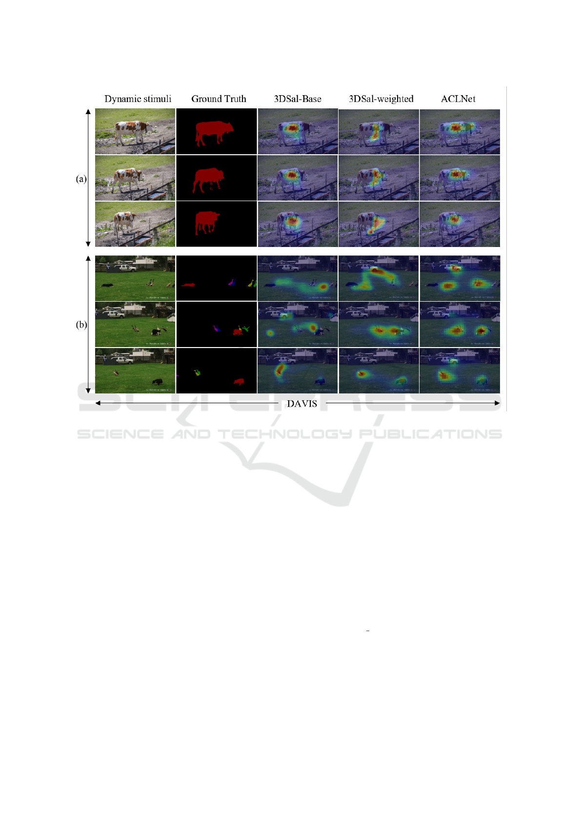
Figure 4: Qualitative results of our 3DSAL model and the ACLNet model (Wang et al., 2018) on two validation video samples

from the object segmentation dataset DAVIS. It can be observed that the proposed 3DSAL-weighted is able to capture the main

objects in the scene.

tiveness of 3D convolutions to capture motion.

•

In Fig. 5, it is noticeable that the generated saliency

maps using 3DSAL-base are sparse, this is due to

the large number of features in the latent space,

the model tends to give a high probability to a

given pixel, which makes it salient. In the 3DSAL-

weighted version, the use of the weighting function

forces the model to generate a more focused and

consistent saliency regions.

5 CONCLUSION

In this paper, we target the problem of learning spatio-

temporal features for video saliency prediction using

3D ConvNets, trained on large-scale video saliency

datasets. We proposed the 3DSAL-weighted video

saliency model, which fuses the spatio-temporal fea-

tures from adjacent frames to accurately learn the hid-

den relationship that affects human behavior when

watching videos. We extensively tested the perfor-

mance of our model on: DHF1K, UFC-SPORT and

DAVIS datasets, and reported the performance of

our model compared with the state-of-the-art video

saliency models. It is worth noting the competitive-

ness of the proposed model, whereby results on UFC-

SPORT dataset outperform the state-of-the-art models.

ACKNOWLEDGEMENT

The authors gratefully acknowledge the support of

Ericsson Algeria for the donation of GPUs used in

this work. This material is based on works sup-

ported by Science Foundation Ireland under Grant No.

SFI/12/RC/2289 P2.

3DSAL: An Efﬁcient 3D-CNN Architecture for Video Saliency Prediction

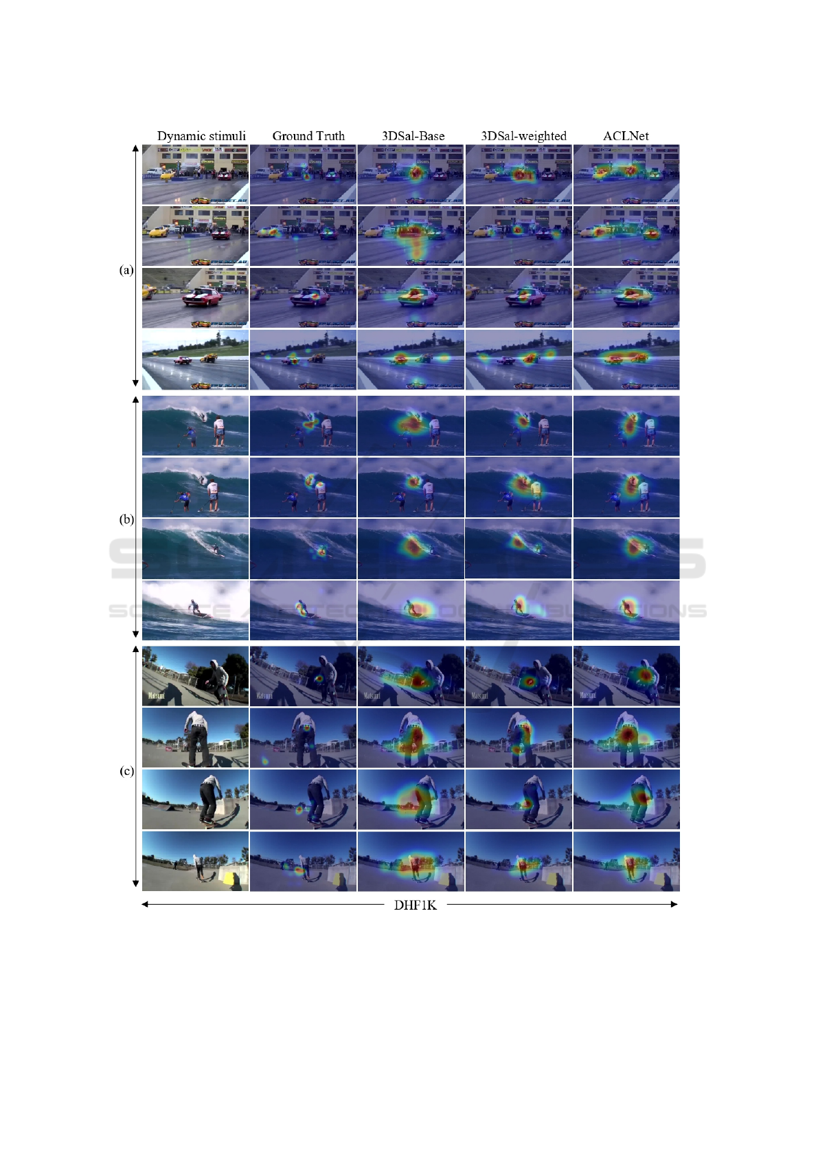
Figure 5: Qualitative results of our 3DSal model and ACLNet (Wang et al., 2018) on three validation video samples from

DHF1K dataset. It can be observed that the proposed 3DSal-weighted is able to handle various challenging scenes well and

produces consistent video saliency results.

VISAPP 2020 - 15th International Conference on Computer Vision Theory and Applications

REFERENCES

Adel Bargal, S., Zunino, A., Kim, D., Zhang, J., Murino, V.,

and Sclaroff, S. (2018). Excitation backprop for rnns.

In Proceedings of the IEEE Conference on Computer

Vision and Pattern Recognition, pages 1440–1449.

Bak, C., Kocak, A., Erdem, E., and Erdem, A. (2018). Spatio-

temporal saliency networks for dynamic saliency pre-

diction. IEEE Transactions on Multimedia, 20(7):1688–

1698.

Borji, A. (2018). Saliency prediction in the deep learn-

ing era: An empirical investigation. arXiv preprint

arXiv:1810.03716.

Borji, A. and Itti, L. (2013). State-of-the-art in visual atten-

tion modeling. IEEE transactions on pattern analysis

and machine intelligence, 35(1):185–207.

Borji, A. and Itti, L. (2015). Cat2000: A large scale ﬁxation

dataset for boosting saliency research. arXiv preprint

arXiv:1505.03581.

Bruce, N. and Tsotsos, J. (2006). Saliency based on informa-

tion maximization. In Advances in neural information

processing systems, pages 155–162.

Bylinskii, Z., Judd, T., Borji, A., Itti, L., Durand, F., Oliva,

A., and Torralba, A. Mit saliency benchmark.

Cornia, M., Baraldi, L., Serra, G., and Cucchiara, R. (2016).

A deep multi-level network for saliency prediction. In

2016 23rd International Conference on Pattern Recog-

nition (ICPR), pages 3488–3493. IEEE.

Deng, J., Dong, W., Socher, R., Li, L.-J., Li, K., and Fei-Fei,

L. (2009). Imagenet: A large-scale hierarchical image

database. In 2009 IEEE conference on computer vision

and pattern recognition, pages 248–255. Ieee.

Gao, D. and Vasconcelos, N. (2005). Discriminant saliency

for visual recognition from cluttered scenes. In Ad-

vances in neural information processing systems, pages

481–488.

Garcia-Diaz, A., Fdez-Vidal, X. R., Pardo, X. M., and Dosil,

R. (2009). Decorrelation and distinctiveness provide

with human-like saliency. In International Conference

on Advanced Concepts for Intelligent Vision Systems,

pages 343–354. Springer.

Garcia-Diaz, A., Fdez-Vidal, X. R., Pardo, X. M., and

Dosil, R. (2012). Saliency from hierarchical adapta-

tion through decorrelation and variance normalization.

Image and Vision Computing, 30(1):51–64.

Goferman, S., Zelnik-Manor, L., and Tal, A. (2012). Context-

aware saliency detection. IEEE transactions on pattern

analysis and machine intelligence, 34(10):1915–1926.

Goodfellow, I., Pouget-Abadie, J., Mirza, M., Xu, B., Warde-

Farley, D., Ozair, S., Courville, A., and Bengio, Y.

(2014). Generative adversarial nets. In Advances in

neural information processing systems, pages 2672–

2680.

Guo, C., Ma, Q., and Zhang, L. (2008). Spatio-temporal

saliency detection using phase spectrum of quaternion

fourier transform. In 2008 IEEE Conference on Com-

puter Vision and Pattern Recognition, pages 1–8. IEEE.

Hochreiter, S. and Schmidhuber, J. (1997). Long short-term

memory. Neural computation, 9(8):1735–1780.

Hossein Khatoonabadi, S., Vasconcelos, N., Bajic, I. V., and

Shan, Y. (2015). How many bits does it take for a

stimulus to be salient? In Proceedings of the IEEE

Conference on Computer Vision and Pattern Recogni-

tion, pages 5501–5510.

Huang, X., Shen, C., Boix, X., and Zhao, Q. (2015). Salicon:

Reducing the semantic gap in saliency prediction by

adapting deep neural networks. In Proceedings of the

IEEE International Conference on Computer Vision,

pages 262–270.

Itti, L., Koch, C., and Niebur, E. (1998). A model of saliency-

based visual attention for rapid scene analysis. IEEE

Transactions on Pattern Analysis & Machine Intelli-

gence, (11):1254–1259.

Ji, S., Xu, W., Yang, M., and Yu, K. (2013). 3d convolu-

tional neural networks for human action recognition.

IEEE transactions on pattern analysis and machine

intelligence, 35(1):221–231.

Jiang, L., Xu, M., Liu, T., Qiao, M., and Wang, Z. (2018a).

Deepvs: A deep learning based video saliency pre-

diction approach. In The European Conference on

Computer Vision (ECCV).

Jiang, L., Xu, M., Liu, T., Qiao, M., and Wang, Z. (2018b).

Deepvs: A deep learning based video saliency predic-

tion approach. In Proceedings of the European Confer-

ence on Computer Vision (ECCV), pages 602–617.

Jiang, L., Xu, M., and Wang, Z. (2017). Predicting video

saliency with object-to-motion cnn and two-layer con-

volutional lstm. arXiv preprint arXiv:1709.06316.

Jiang, M., Huang, S., Duan, J., and Zhao, Q. (2015). Sali-

con: Saliency in context. In The IEEE Conference on

Computer Vision and Pattern Recognition (CVPR).

Judd, T., Durand, F., and Torralba, A. (2012). A benchmark

of computational models of saliency to predict human

ﬁxations.

Kingma, D. P. and Ba, J. (2014). Adam: A

method for stochastic optimization. arXiv preprint

arXiv:1412.6980.

Kruthiventi, S. S., Ayush, K., and Babu, R. V. (2017). Deep-

ﬁx: A fully convolutional neural network for predicting

human eye ﬁxations. IEEE Transactions on Image Pro-

cessing, 26(9):4446–4456.

ummerer, M., Theis, L., and Bethge, M. (2014). Deep

gaze i: Boosting saliency prediction with feature maps

trained on imagenet. arXiv preprint arXiv:1411.1045.

Leboran, V., Garcia-Diaz, A., Fdez-Vidal, X. R., and Pardo,

X. M. (2017). Dynamic whitening saliency. IEEE

transactions on pattern analysis and machine intelli-

gence, 39(5):893–907.

Leifman, G., Rudoy, D., Swedish, T., Bayro-Corrochano,

E., and Raskar, R. (2017). Learning gaze transitions

from depth to improve video saliency estimation. In

Proceedings of the IEEE International Conference on

Computer Vision, pages 1698–1707.

Li, X., Zhao, L., Wei, L., Yang, M.-H., Wu, F., Zhuang,

Y., Ling, H., and Wang, J. (2016). Deepsaliency:

Multi-task deep neural network model for salient object

detection. IEEE Transactions on Image Processing,

25(8):3919–3930.

3DSAL: An Efﬁcient 3D-CNN Architecture for Video Saliency Prediction

Linardos, P., Mohedano, E., Cherto, M., Gurrin, C., and

i Nieto, X. G. (2018). Temporal saliency adaptation in

egocentric videos.

Liu, N., Han, J., Zhang, D., Wen, S., and Liu, T. (2015).

Predicting eye ﬁxations using convolutional neural net-

works. In Proceedings of the IEEE Conference on

Computer Vision and Pattern Recognition, pages 362–

370.

Mancas, M., Ferrera, V. P., Riche, N., and Taylor, J. G.

(2016). From Human Attention to Computational At-

tention, volume 2. Springer.

Mathe, S. and Sminchisescu, C. (2015). Actions in the

eye: Dynamic gaze datasets and learnt saliency models

for visual recognition. IEEE transactions on pattern

analysis and machine intelligence, 37(7):1408–1424.

Mital, P. K., Smith, T. J., Hill, R. L., and Henderson, J. M.

(2011). Clustering of gaze during dynamic scene view-

ing is predicted by motion. Cognitive Computation,

3(1):5–24.

Nwankpa, C., Ijomah, W., Gachagan, A., and Marshall, S.

(2018). Activation functions: Comparison of trends

in practice and research for deep learning. CoRR,

abs/1811.03378.

Pan, J., Ferrer, C. C., McGuinness, K., O’Connor, N. E., Tor-

res, J., Sayrol, E., and Giro-i Nieto, X. (2017). Salgan:

Visual saliency prediction with generative adversarial

networks. arXiv preprint arXiv:1701.01081.

Pan, J., Sayrol, E., Giro-i Nieto, X., McGuinness, K., and

O’Connor, N. E. (2016). Shallow and deep convolu-

tional networks for saliency prediction. In Proceedings

of the IEEE Conference on Computer Vision and Pat-

tern Recognition, pages 598–606.

Perazzi, F., Pont-Tuset, J., McWilliams, B., Van Gool, L.,

Gross, M., and Sorkine-Hornung, A. (2016). A bench-

mark dataset and evaluation methodology for video

object segmentation. In Proceedings of the IEEE Con-

ference on Computer Vision and Pattern Recognition,

pages 724–732.

Prechelt, L. (1998). Early stopping-but when? In Neural

Networks: Tricks of the trade, pages 55–69. Springer.

Rudoy, D., Goldman, D. B., Shechtman, E., and Zelnik-

Manor, L. (2013). Learning video saliency from hu-

man gaze using candidate selection. In Proceedings of

the IEEE Conference on Computer Vision and Pattern

Recognition, pages 1147–1154.

Saslow, M. (1967). Effects of components of displacement-

step stimuli upon latency for saccadic eye movement.

Josa, 57(8):1024–1029.

Seo, H. J. and Milanfar, P. (2009). Static and space-time

visual saliency detection by self-resemblance. Journal

of vision, 9(12):15–15.

Simonyan, K. and Zisserman, A. (2014). Very deep con-

volutional networks for large-scale image recognition.

arXiv preprint arXiv:1409.1556.

Tran, D., Bourdev, L., Fergus, R., Torresani, L., and Paluri,

M. (2015). Learning spatiotemporal features with 3d

convolutional networks. In Proceedings of the IEEE

international conference on computer vision, pages

4489–4497.

Vig, E., Dorr, M., and Cox, D. (2014). Large-scale optimiza-

tion of hierarchical features for saliency prediction in

natural images. In Proceedings of the IEEE Conference

on Computer Vision and Pattern Recognition, pages

2798–2805.

Wang, W., Shen, J., Guo, F., Cheng, M.-M., and Borji, A.

(2018). Revisiting video saliency: A large-scale bench-

mark and a new model. In Proceedings of the IEEE

Conference on Computer Vision and Pattern Recogni-

tion, pages 4894–4903.

Xu, M., Jiang, L., Sun, X., Ye, Z., and Wang, Z. (2017).

Learning to detect video saliency with hevc features.

IEEE Transactions on Image Processing, 26(1):369–

385.

Zhang, J. and Sclaroff, S. (2013). Saliency detection: A

boolean map approach. In Proceedings of the IEEE

international conference on computer vision, pages

153–160.

VISAPP 2020 - 15th International Conference on Computer Vision Theory and Applications