
Influence of Data Similarity on the Scoring Power of
Machine-learning Scoring Functions for Docking
Kam-Heung Sze
1
, Zhiqiang Xiong
1
, Jinlong Ma
1
, Gang Lu
2
, Wai-Yee Chan
2
and Hongjian Li
1,2*
1
Bioinformatics Unit, SDIVF R&D Centre, Hong Kong Science Park, Sha Tin, New Territories, Hong Kong
2
CUHK-SDU Joint Laboratory on Reproductive Genetics, School of Biomedical Sciences,
The Chinese University of Hong Kong, Sha Tin, New Territories, Hong Kong
Keywords: Molecular Docking, Binding Affinity Prediction, Machine Learning, Feature Engineering, Data Similarity.
Abstract: Inconsistent conclusions have been drawn from recent studies exploring the influence of data similarity on
the scoring power of machine-learning scoring functions, but they were all based on the PDBbind v2007
refined set whose data size is limited to just 1300 protein-ligand complexes. Whether these conclusions can
be generalized to substantially larger and more diverse datasets warrants further examinations. Besides, the
previous definition of protein structure similarity, which relied on aligning monomers, might not truly reflect
what it was supposed to be. Moreover, the impact of binding pocket similarity has not been investigated either.
Here we have employed the updated refined set v2013 providing 2959 complexes and utilized not only protein
structure and ligand fingerprint similarity but also a novel measure based on binding pocket topology
dissimilarity to systematically control how similar or dissimilar complexes are incorporated for training
predictive models. Three empirical scoring functions X-Score, AutoDock Vina, Cyscore and their random
forest counterparts were evaluated. Results have confirmed that dissimilar training complexes may be
valuable if allied with appropriate machine learning algorithms and informative descriptor sets. Machine-
learning scoring functions acquire their remarkable scoring power through mining more data to advance
performance persistently, whereas classical scoring functions lack such learning ability. The software code
and data used in this study and supplementary results are available at https://GitHub.com/HongjianLi/MLSF.
1 INTRODUCTION
In structural bioinformatics, the prediction of binding
affinity of a protein-ligand complex is carried out by
a scoring function (SF). In contrast to the classical
SFs which rely on linear regression using a carefully
selected array of molecular descriptors driven by
expert knowledge, machine-learning SFs circumvent
such predetermined functional forms and instead
infer a vastly nonlinear model from the data. Various
studies have already illustrated the remarkable
performance of machine-learning SFs over classical
SFs (Ain et al., 2015; Li et al., 2017).
Controversy over the influence of data similarity
between the training and test sets on the scoring
power of SFs has arisen lately. Li and Yang
quantified the training-test set similarity in terms of
protein structures and sequences, and used the
similarity cutoffs to split the full training set into a
series of nested training sets, showing that machine-
learning SFs failed to outperform classical SFs after
removal of training complexes whose proteins are
greatly similar to the test proteins identified by
structure alignment and sequence alignment, leading
to the conclusion that the outstanding scoring power
of machine-learning SFs is exclusively attributed to
the presence of training complexes with highly
similar proteins to those in the test set (Li and Yang,
2017). However, a follow-up but expanded re-
analysis by Li et al. revealed instead that even when
trained with a moderate percent of dissimilar proteins
machine-learning SFs would already outperform
classical SFs, leading to the different conclusion that
machine-learning SFs owe a considerable portion of
their superior performance to training on complexes
with dissimilar proteins to those in the test set (Li et
al., 2018). Subsequently the same authors further
demonstrated that classical SFs are unable to exploit
large capacities of structural and interaction data, as
incorporating a larger proportion of similar
complexes to the training set did not render classical
SFs more accurate (Li et al., 2019).
Sze, K., Xiong, Z., Ma, J., Lu, G., Chan, W. and Li, H.
Influence of Data Similarity on the Scoring Power of Machine-learning Scoring Functions for Docking.
DOI: 10.5220/0008873800850092
In Proceedings of the 13th International Joint Conference on Biomedical Engineering Systems and Technologies (BIOSTEC 2020) - Volume 3: BIOINFORMATICS, pages 85-92
ISBN: 978-989-758-398-8; ISSN: 2184-4305
Copyright
c
2022 by SCITEPRESS – Science and Technology Publications, Lda. All rights reserved
85

To deeply elaborate how SFs would behave given
varying degrees of data similarity, here we are
revisiting this interesting question with an extensively
revised methodology in the following ways. First, all
the above-mentioned three studies employed
PDBbind v2007 refined set as the solo benchmark,
which is limited to a small amount of merely 1300
complexes. It remains unclear whether the impact of
data similarity on SFs would be generalizable to
larger datasets. Therefore we will employ the updated
v2013 benchmark (Li et al., 2014) offering 2959
complexes, whose data size has more than doubled.
Second, in the above studies the structural similarity
between a pair of training and test set proteins was
defined as the TM-score calculated from the structure
alignment program TM-align, but TM-align can only
be applied to aligning a single-chain structure to
another single-chain structure. Given that most
proteins of the PDBbind benchmarks contain multiple
chains, each chain was extracted and compared. This
all-chains-against-all-chains method, despite being
convenient, could possibly step into the danger of
misaligning to an irrelevant chain. Thus, we will
switch to MM-align (Mukherjee and Zhang, 2009),
which is specifically designed for structurally
aligning multiple-chain protein-protein complexes.
Moreover, the similarity of two complexes is
determined by not only their proteins in global shape
but also their ligands in local binding sites, hence we
will supplement a novel similarity measure based on
pocket topology.
2 METHODS
2.1 Performance Benchmark
The PDBbind benchmarks have been widely used for
evaluating the scoring power of SFs. Here v2013 was
exploited, whose refined set provides 2959 crystal
structures of protein-ligand complexes as well as their
experimentally measured binding affinities. Among
them, a core set of 195 complexes were usually
reserved for test purpose, and the remaining 2764
complexes were used for training. Although v2013
happens to have a core set of the same size as that of
v2007, only 25 (13%) complexes are identical,
whereas the other 170 (87%) complexes are new and
not included for evaluation in the recent three studies.
As usual, three quantitative indicators of the scoring
power, namely root mean square error (RMSE),
Pearson correlation coefficient (Rp) and Spearman
correlation coefficient (Rs), were employed to assess
the predictive accuracy of the considered SFs.
2.2 Similarity Measures
There are multiple ways to define the similarity of a
training complex and a test complex, either by their
proteins, their ligands, or their binding pockets.
Previously the structural similarity of two proteins
was defined as the TM-score, which has the value in
(0,1]. The TM-score was computed by the TM-align
program which generates an optimized residue-to-
residue alignment for comparing two protein chains
whose sequences can be different. Nevertheless, TM-
align is limited to aligning single-chain monomer
protein structures. On the contrary, MM-align is
purposely designed for aligning multiple-chain
multimer protein structures. It is built on a heuristic
iteration of a modified Needleman-Wunsch dynamic
programming algorithm, with the alignment score
specified by the inter-complex residue distances. The
multiple chains in each complex are joined in every
possible order and then simultaneously aligned with
cross-chain alignments prevented. The TM-score
reported by MM-align after being normalized by the
test protein was used to define the protein structure
similarity here, thus avoiding the risk of misaligning
a chain of a protein to an irrelevant chain in another
protein.
Likewise, the similarity of binding ligands of the
training and test sets were also taken into account by
calculating the ECFP4 fingerprint implemented in
OpenBabel and their pairwise Tanimoto coefficients.
Such ligand fingerprint similarity was not explicitly
used to create a series of nested training sets in two
previous studies (Li and Yang, 2017; Li et al., 2018),
but here it is devoted to offer a comparison to protein
structure similarity.
The similarity of binding pockets of training and
test sets is investigated for the first time in the present
study. While the protein structure similarity is of
global nature, i.e. it considers the whole protein
structure when calculating structural similarity, the
binding of a ligand to a macromolecular protein is
instead mostly determined by the local environment
of the binding pocket. In fact, the same ligand–
binding domain may be found in globally dissimilar
proteins. This explains the rationale of supplementing
such an extra similarity measure. To implement, the
TopMap algorithm (ElGamacy and Van Meervelt,
2015) was applied on the pocket of each protein to
encode its geometrical shape and atomic partial
charges into a feature vector of fifteen numeric
elements. The dissimilarity of two comparing pockets
was then quantified as the Manhattan distance
between their feature vectors. Pay attention that the
dissimilarity calculated by TopMap does not get
BIOINFORMATICS 2020 - 11th International Conference on Bioinformatics Models, Methods and Algorithms
86

transformed to a normalized similarity value with
either a generalized exponential function or a
generalized Lorentz function. Hence the larger the
dissimilarity value is, the more dissimilar the two
comparing pockets are.
Having the three similarity measures properly
defined, nested sets of training complexes with
increasing degree of similarity to the test set were
created as follows. At a certain cutoff, a complex is
included in the training set if its similarity to every
test complex is always no greater than the cutoff
value. In other words, a training complex is excluded
from the original full training set if its similarity to
any of the test complexes is higher than the cutoff.
Mathematically, given a fixed test set (TS), for both
protein structure similarity and ligand fingerprint
similarity whose values are normalized to [0, 1], a
series of new training sets (NT) were constructed
through gradually accumulating samples from the
original training set (OT) according to varying
similarity cutoff values:
|
∈∀
∈,
,
(1)
where
and
represent the ith and jth samples
from OT and TS, respectively;
,
is the
similarity between
and
; and c is the similarity
cutoff used to control the generation of new training
sets. By definition,
0
∅,
1 .
When the cutoff value c steadily increases from 0 to
1, nested sets of training complexes with increasing
degrees of similarity to the test set were accordingly
created. Analogously in an opposite direction, nested
sets of training complexes with increasing degrees of
dissimilarity to the test set were created as follows,
but this time with the cutoff value c steadily
decreasing from 1 to 0:
|
∈∃
∈,
,
(2)
By definition,
1
∅,
0
. Indeed,
∀ ∈
0, 1
,
∪
,
∩
∅.
Note that the above equations apply to protein
structure and ligand fingerprint similarity measures
only. In the case of pocket topology, as the values
indicate dissimilarity rather than similarity and they
fall in the range of [0, +∞), a slightly different
definition is required to construct nested training sets
with increasing degrees of similarity to the test set
when the cutoff c steadily decreases from +∞ to 0:
|
∈∀
∈,
,
(3)
where
,
is the dissimilarity between
and
. Analogously in an opposite direction, nested
sets of training complexes with increasing degrees of
dissimilarity to the test set were created as follows
with c steadily increasing from 0 to +∞:
|
∈∃
∈,
,
(4)
Likewise by definition, ∀ ∈
0, ∞
,
∪
,
∩
∅.
2.3 Scoring Functions
Classical SFs taking on multiple linear regression
(MLR) were compared to their machine-learning
counterparts. X-Score (Wang et al., 2002) v1.3 was
selected as a representative of classical SFs because
on the PDBbind v2013 core set it performed the best
among a panel of 20 SFs, most of which are
implemented in mainstream commercial software. X-
Score is a consensus of three constituent scores which
all consider four common intermolecular features:
van der Waals interaction (VDW), hydrogen bonding
(HB), deformation penalty (RT), and hydrophobic
effect (HP/HM/HS). The three parallel SFs only
differ in the computation of the hydrophobic effect
term. To rebuild X-Score, the three constituent SFs
were individually trained using MLR with
coefficients for each score re-calibrated on the new
training sets with similarity control. To build a
machine-learning counterpart, the same six
descriptors were fed to random forest (RF), thereby
generating RF::Xscore.
Provided that X-Score is a SF dated back in 2002
which might not reflect the latest development in this
area, the recent classical SFs AutoDock Vina (Trott
and Olson, 2010) v1.1.2 and Cyscore (Cao and Li,
2014) v2.0.3 as well as their random forest variants
RF::Vina (Li et al., 2015) and RF::Cyscore (Li et al.,
2014) were also built and evaluated.
Furthermore, as machine learning algorithms can
easily incorporate more variables for training, the six
descriptors from X-Score, the six descriptors from
Vina and the four descriptors from Cyscore were
combined to spawn a novel machine-learning SFs,
RF::XVC, to investigate to what extent the mixed
descriptors would contribute to the performance
compared to RF::Xscore, RF::Vina and RF::Cyscore.
Influence of Data Similarity on the Scoring Power of Machine-learning Scoring Functions for Docking
87

3 RESULTS AND DISCUSSION
First, we had to determine specific cutoff values to
systematically adjust how similar or dissimilar
complexes are incorporated for training. We tried
different settings and consequently decided that, for
protein structure similarity, the cutoff value c
increases from 0.40 to 1.00 with a step size of 0.01 in
the direction specified by
, and decreases from
0.99 to 0.40 and then to 0 in the opposite direction
specified by
; for ligand fingerprint similarity, c
increases from 0.55 to 1.00 in
, and decreases
from 0.99 to 0.55 and then to 0 in
; for pocket
topology dissimilarity, c decreases from 10.0 to 0
with a step size of 0.2 in
, and increases from 0.2
to 10.0 and then to +∞ in
.
Next, we plotted the number of training
complexes against the three types of cutoff (Figure 1),
in order to visibly show that these distributions are
hardly even. In fact, the distribution of training
complexes under the protein structure similarity
measure is extraordinarily skewed, e.g. as many as
859 training complexes (accounting for 31% of the
original full training set of 2764 complexes) have a
test set similarity greater than 0.99 (note the sheer
height of the rightmost bar), and 156 training
complexes have a test set similarity in the range of
(0.98, 0.99]. Incrementing the cutoff by just 0.01 from
0.99 to 1.00 will include 859 additional training
complexes, whereas incrementing the cutoff by the
same step size from 0.90 to 0.91 will include merely
17 additional training complexes, even none from
0.72 to 0.73. Therefore, one would seemingly expect
a significant performance gain from raising the cutoff
by just 0.01 if the cutoff is already at 0.99. This is also
true, although less apparent, for ligand fingerprint
similarity, where 179 training complexes have a test
set similarity greater than 0.99. The distribution under
the pocket topology dissimilarity measure, however,
seems relatively more uniform, with just 15
complexes falling in the range of [0, 0.2) and just 134
complexes in the range of [10, +∞). Hence
introducing this supplementary similarity measure
based on pocket topology, which is novel in this study,
offers a different tool to investigate the influence of
data similarity on the scoring power of SFs with
training set size unbiased towards both ends of cutoff.
Keeping in mind the above-illustrated non-even
distributions, we re-trained the three classical SFs
(MLR::Xscore, MLR::Vina, MLR::Cyscore) and the
four machine-learning SFs (RF::Xscore, RF::Vina,
RF::Cyscore, RF::XVC) on the 61 nested training sets
generated with protein structure similarity measure,
evaluated their scoring power on the PDBbind v2013
core set, and plotted their predictive performance (in
terms of Rp, Rs and RMSE) in a consistent scale
against both cutoff value and number of training
complexes in two similarity directions (Figure 2).
Looking at the top row alone, where RF::Xscore was
not able to surpass MLR::Xscore until the similarity
cutoff reached 0.99, it is therefore not surprising for
Li and Yang to draw their conclusion that after
removal of training proteins that are highly similar to
the test proteins, machine-learning SFs did not
outperform classical SFs in Rp (Li and Yang, 2017)
(note that the v2007 dataset employed in previous
studies has an analogously skewed distribution as the
v2013 dataset employed in this study; data not
shown). Nonetheless, if one looks at the second row,
which plots essentially the same result but against the
associated number of training complexes instead, it
becomes clear that RF::Xscore trained on 1905 (the
number of training complexes associated to cutoff
0.99, about 69% of the full 2764 complexes)
complexes was able to outperform MLR::Xscore,
which was already the best performing classical SF
considered here. In terms of RMSE, RF::Xscore
surpassed MLR::Xscore at cutoff=0.91 when they
were trained on just 1458 (53%) complexes whose
proteins are not so similar to those in the test set. This
is more apparent for RF::XVC, which outperformed
MLR::Xscore at a cutoff of just 0.70, corresponding
to only 1243 (45%) training complexes. In other
words, even if the original training set was split into
two halves and the half with proteins dissimilar to the
test set was used for training, machine-learning SFs
would still produce a smaller prediction error than the
best classical SF. Having said that, it does not make
sense for anyone to exclude the most relevant samples
for training (Li et al., 2018). When the full training set
was used, a large performance gap between machine-
learning and classical SFs was observed. From a
different viewpoint, through comparing the top two
rows showing basically the same result but with
different horizontal axis, the crossing point where
RF::Xscore started to overtake MLR::Xscore is
located near the right edge of the subfigures in the
first row, whereas the same crossing point is
noticeably left shifted in the second row, suggesting
that the outstanding scoring power of RF::Xscore and
RF::XVC is actually attributed to increasing training
set size but not exclusively to a high similarity cutoff
value as claimed previously.
Due to the skewness of the distribution of training
complexes under the protein structure similarity
measure, it should be understandable to anticipate a
remarkable performance gain from raising the cutoff
by only 0.01 if it already touches 0.99 because it will
BIOINFORMATICS 2020 - 11th International Conference on Bioinformatics Models, Methods and Algorithms
88
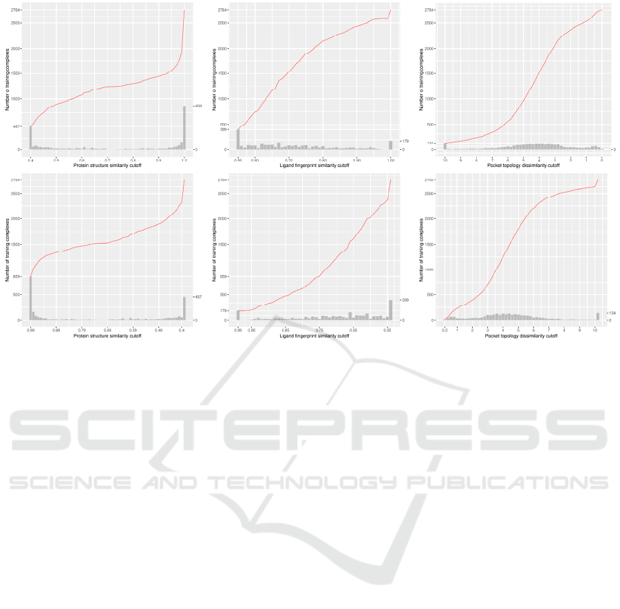
Figure 1: Number of training complexes against protein structure similarity cutoff (left column), ligand fingerprint similarity
cutoff (center column) and pocket topology dissimilarity cutoff (right column) in two directions, either starting from a small
training set comprising complexes most dissimilar to the test set (top row) or starting from a small training set comprising
complexes most similar to the test set (bottom row). The histogram plots the number of additional complexes that will be
added to a larger set when the protein structure similarity cutoff is incremented by the step size of 0.01 (left), when the ligand
fingerprint similarity cutoff is incremented by 0.01 (center), or when the pocket topology dissimilarity cutoff is decremented
by 0.2 (right). Hence the number of training complexes referenced by an arbitrary point of the red curve is equal to the
cumulative summation over the heights of all the bars of and before the corresponding cutoff. By definition, the histogram of
the three subfigures at the bottom row is identical to the histogram at the top row after being mirrored along the median cutoff.
incorporate as many as 859 complexes whose
proteins are the most similar to those in the test set.
However, this is only true for machine-learning SFs
but false for classical SFs. The Rp for RF::Xscore,
RF::Vina and RF::XVC notably increased from
0.642, 0.640 and 0.660 to 0.658, 0.683 and 0.714,
respectively, and their RMSE reduced from 1.74, 1.75
and 1.72 to 1.72, 1.69 and 1.63, respectively. By
contrast, the performance of classical SFs even
worsened a little bit, raising RMSE from 1.79 to 1.81
for MLR::Xscore and degrading Rp from 0.620 to
0.603 for MLR::Cyscore. Feeding the most relevant
data to train MLR models surprisingly cost them to
be even less accurate.
Among the three classical SFs, MLR::Xscore was
the most predictive, followed by MLR::Cyscore.
MLR::Vina performed substantially worse because
the Nrot term was not re-optimized provided that no
optimization detail was disclosed by the original
authors. Hence MLR::Vina in principle served as a
baseline model for comparison. It is important to
witness that their performance stagnated and could
not benefit from more training data, even those that
are most relevant to the test set. In line with the
conclusion by Li et al., classical SFs are unable to
exploit large volumes of structural and interaction
data (Li et al., 2019) because of insufficient model
complexity with few parameters and imposition of a
fixed functional form. This is a critical disadvantage
of classical SFs because more and more structural and
interaction data will be available in the future and
these SFs cannot properly exploit such big data.
RF::XVC, empowered by its integration of
features from all three individual SFs, undoubtedly
turned out to be the best performing machine-learning
SF, followed by RF::Vina and RF::Xscore.
RF::Cyscore somewhat underperformed and failed to
match its performance to RF::Vina or RF::Xscore.
We suspect a possible reason could be the lack of
adequate distinguishing power of two of the four
descriptors used by Cyscore (hydrogen-bond energy
and the ligand's entropy) during RF construction, as
their variable importance had been previously shown
to be significantly low, reflected by the percentage of
Influence of Data Similarity on the Scoring Power of Machine-learning Scoring Functions for Docking
89
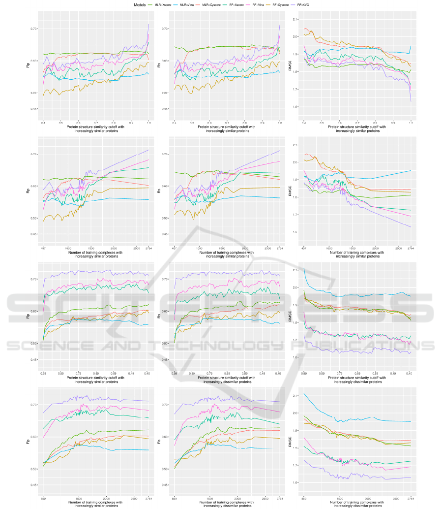
Figure 2: Scoring power of three classical SFs (MLR::Xscore, MLR::Vina and MLR::Cyscore) and four machine-learning
SFs (RF::Xscore, RF::Vina, RF::Cyscore and RF::XVC) evaluated on the PDBbind v2013 benchmark when they were built
on nested training sets generated with protein structure similarity measure. The left, center and right columns demonstrate the
predictive performance of the considered SFs in terms of Rp, Rs and RMSE, respectively. The first row plots the performance
against cutoff, whereas the second row plots essentially the same result but against the associated number of training
complexes instead. Both rows present the result where training complexes were formed by proteins that were firstly most
dissimilar to those in the test set and then progressively expanded to incorporate similar proteins as well. The bottom two
rows, conversely, depict the performance in a reversed similarity direction where only training complexes similar to those in
the test set were exploited initially and then dissimilar complexes were gradually included as well.
BIOINFORMATICS 2020 - 11th International Conference on Bioinformatics Models, Methods and Algorithms
90

increase in mean square error observed in out-of-bag
prediction after a particular feature was permuted at
random (Li et al., 2014). Despite being the least
predictive among the group of machine-learning SFs,
RF::Cyscore still possessed the capability of keeping
proliferating performance persistently with more
training data, which was not seen in classical SFs.
Though RF::Cyscore performed far worse than
MLR::Cyscore initially (Rp=0.490 vs 0.563), with
this learning capability it kept improving and finally
managed to yield a comparable Rp value on the full
training set (0.594 vs 0.603) and produce an even
lower RMSE value (1.83 vs 1.84).
From the top two rows of Figure 2 we have just
illustrated that RF::XVC already surpassed classical
SFs when trained on just 45% of complexes most
dissimilar to the test set, although this percentage
could be further reduced to 32% if extra sets of
features were put into assessment (Li et al., 2019). We
now inspect a different scenario, represented by the
bottom two rows, where the training set was initially
composed of complexes highly similar to those in the
test set only and regularly enlarged to include
dissimilar complexes as well. In this context, the
curves for RF::XVC, RF::Vina and RF::Xscore are
always above those of the classical SFs in Rp and Rs
and always below in RMSE, indicating the superior
performance of these machine-learning SFs to any of
the classical SFs regardless of the cutoff. This
constitutes a strong result that under no circumstances
did any of the classical SFs outperform any of the
machine-learning SFs (except RF::Cyscore due to the
possible reason explained above). This was one of the
major conclusions made by Li et al. on the v2007
benchmark (Li et al., 2019) and now it is deemed
generalizable to the larger and more diverse v2013
benchmark being investigated here.
Interestingly, unlike in the previous similarity
direction where the peak performance for machine-
learning SFs was achieved by using the full training
set of 2764 complexes, here the peak performance
was obtained at a cutoff of 0.61 (1647 complexes) for
RF::XVC (Rp=0.731, RMSE=1.62), 0.65 (1580
complexes) for RF::Vina (Rp=0.703, RMSE=1.67),
and 0.46 (1990 complexes) for RF::Xscore
(Rp=0.686, RMSE=1.70). Such peak was also
detected on the v2007 benchmark (Li et al., 2019),
and its occurrence seems to be due to a certain
compromise between the training set volume and its
relevance to the test data: incorporating additional
complexes dissimilar to the test set beyond a certain
threshold of similarity cutoff would probably
introduce data noise. That said, the performance
difference between machine-learning SFs trained on
a subset generated from an optimal cutoff and those
trained on the full set is just marginal. For instance,
the RMSE obtained by RF::XVC, RF::Vina and
RF::Xscore trained on the full set was 1.63, 1.69 and
1.72, respectively, pretty close to their peak
performance. Training machine-learning SFs on the
full set of complexes, although being a bit less
predictive compared to training on a prudently
selected subset of complexes most similar to the test
set, has the hidden advantage of possessing the widest
applicability domain, suggesting that such models
should predict better on more diverse test sets
containing protein families not present in the v2013
core set. Moreover, this simple approach of using the
full set for training does not bother to search for the
optimal cutoff value, which does not seem an easy
task. Failing that would probably incur a suboptimal
performance than simply utilizing the full set.
Consistent with the common belief, now validated
again after Li et al.’s study on the v2007 dataset (Li
et al., 2019), training complexes formed by proteins
similar to those in the test set contribute significantly
more to the performance of machine-learning SFs
than proteins dissimilar to the test set. For example,
RF::XVC yielded Rp=0.719, Rs=0.718, RMSE=1.64
when trained on the 1360 complexes (cutoff=0.87)
comprising proteins most similar to the test set, versus
Rp=0.611, Rs=0.609, RMSE=1.82 when the same SF
was trained on the 1360 complexes (cutoff=0.84)
comprising proteins most dissimilar to the test set.
Switching the similarity measure from protein
structure to ligand fingerprint (result at GitHub) also
confirms the above observations. RF::Xscore resulted
in a smaller RMSE than MLR::Xscore at the cutoff
of 0.79 when they were trained on 2083 (75%)
complexes whose ligands are not so similar to those
in the test set. Raising the cutoff by only 0.01 from
0.99 to 1.00, equivalent to incorporating 179
additional training complexes containing ligands
most similar to those in the test set, helped to strongly
boost the performance of machine-learning SFs (Rp
increased from 0.677 to 0.714 for RF::XVC and from
0.643 to 0.683 for RF::Vina) but not classical SFs (Rp
stagnated at 0.622 for MLR::Xscore and slightly
increased from 0.598 to 0.603 for MLR::Cyscore).
Classical SFs were unable to exploit the most relevant
data for training, whereas every machine-learning SF
exhibited the capability of keeping growing
performance consistently with more training data.
Assessed in a reverse similarity direction, the strong
conclusion still holds: under no circumstances did
MLR::Xscore, MLR::Vina or MLR::Cyscore surpass
RF::XVC, RF::Xscore or RF::Vina. The performance
of machine-learning SFs peaked at about 500 to 1000
Influence of Data Similarity on the Scoring Power of Machine-learning Scoring Functions for Docking
91

complexes containing ligands most similar to the test
set, but it is difficult to find such an optimal subset.
Further switching the similarity measure to pocket
topology (result available at GitHub) reveals novel
findings. Recall that under this measure the training
complexes are fairly more evenly distributed among
the dissimilarity cutoff values than the other two
measures (Figure 1). Dropping the cutoff from 0.20
to 0.00 merely introduced 15 additional training
complexes whose pockets are most similar to those in
the test set. To our surprise, including these 15 most
relevant samples in training machine-learning SFs
weakly downgraded the performance of RF::XVC
(Rp dropped from 0.717 to 0.711) and RF::Vina (Rp
dropped from 0.688 to 0.687), but the difference is
insignificant. What is significant is that from the
dissimilarity cutoff range of 6 to 2, among which the
majority of training complexes (1807 or 65%) are
distributed (Figure 1), machine-learning SFs kept
learning and improving performance persistently.
These are not the most relevant data compared to the
397 complexes with a dissimilarity of less than 2, yet
they contributed considerably to the performance of
machine-learning SFs. On the contrary, the
performance of classical SFs nearly levelled off.
4 CONCLUSIONS
Here we have revisited the question of how data
similarity influences the performance of scoring
functions (SFs) on binding affinity prediction. By
systematically evaluating three classical SFs and four
machine-learning SFs on a substantially larger dataset
and using not only protein structure but also ligand
fingerprint and pocket topology for measuring
training-test data similarity, we have confirmed that
dissimilar training complexes may contribute
considerably to the superior performance of machine-
learning SFs (Li et al., 2018; 2019), which is not
exclusively due to inclusion of the most relevant data
as claimed recently (Li and Yang, 2017). These SFs
keep learning with more data and improving scoring
power steadily. Training data most relevant to the test
set contribute substantially more to the predictive
performance of machine-learning SFs than those
most irrelevant to the test set. Training machine-
learning SFs on all the available complexes, despite
not being the most predictive when compared to
training on a certain subset of complexes which has
to be wisely selected, will broaden the applicability
domain and should therefore lead to better result if
evaluated on external benchmarks comprising new
complexes not included in the current benchmark.
ACKNOWLEDGEMENTS
We thank SDIVF R&D Centre for providing a project
grant (SDIVF-PJ-B-18005) to carry out this work.
REFERENCES
Ain, Q.U. et al. (2015) Machine-learning scoring functions
to improve structure-based binding affinity prediction
and virtual screening. Wiley Interdiscip. Rev. Comput.
Mol. Sci., 5, 405–424.
Cao, Y. and Li,L. (2014) Improved protein-ligand binding
affinity prediction by using a curvature-dependent
surface-area model. Bioinformatics, 30, 1674–1680.
ElGamacy, M. and Van Meervelt,L. (2015) A fast
topological analysis algorithm for large-scale similarity
evaluations of ligands and binding pockets. J.
Cheminform., 7, 42.
Li, H. et al. (2019) Classical scoring functions for docking
are unable to exploit large volumes of structural and
interaction data. Bioinformatics, btz183.
Li, H. et al. (2017) Identification of Clinically Approved
Drugs Indacaterol and Canagliflozin for Repurposing to
Treat Epidermal Growth Factor Tyrosine Kinase
Inhibitor-Resistant Lung Cancer. Front. Oncol., 7, 288.
Li, H. et al. (2015) Improving autodock vina using random
forest: The growing accuracy of binding affinity
prediction by the effective exploitation of larger data
sets. Mol. Inform., 34, 115–126.
Li, H., Leung,K.S., et al. (2014) Substituting random forest
for multiple linear regression improves binding affinity
prediction of scoring functions: Cyscore as a case study.
BMC Bioinformatics, 15, 1–12.
Li, H. et al. (2018) The impact of protein structure and
sequence similarity on the accuracy of machine-
learning scoring functions for binding affinity
prediction. Biomolecules, 8, 12.
Li, Y., Liu,Z., et al. (2014) Comparative assessment of
scoring functions on an updated benchmark: 1.
compilation of the test set. J. Chem. Inf. Model., 54,
1700–1716.
Li,Y. and Yang,J. (2017) Structural and Sequence
Similarity Makes a Significant Impact on Machine-
Learning-Based Scoring Functions for Protein-Ligand
Interactions. J. Chem. Inf. Model., 57, 1007–1012.
Mukherjee, S. and Zhang,Y. (2009) MM-align: A quick
algorithm for aligning multiple-chain protein complex
structures using iterative dynamic programming.
Nucleic Acids Res., 37, e83.
Trott, O. and Olson,A.J. (2010) AutoDock Vina: Improving
the speed and accuracy of docking with a new scoring
function, efficient optimization, and multithreading. J.
Comput. Chem., 31, 455–461.
Wang, R. et al. (2002) Further development and validation
of empirical scoring functions for structure-based
binding affinity prediction. J. Comput. Aided. Mol.
Des., 16, 11–26.
BIOINFORMATICS 2020 - 11th International Conference on Bioinformatics Models, Methods and Algorithms
92
