
Trajectory Extraction and Deep Features for Classification of Liquid-gas
Flow under the Context of Forced Oscillation
Luong Phat Nguyen
1
, Julien Mille
1,2
, Dominique Li
1
, Donatello Conte
1
and Nicolas Ragot
1
1
Universit
´
e de Tours, Tours, France
2
INSA Centre Val de Loire, Blois, France
{dominique.li, donatello.conte, nicolas.ragot}@univ-tours.fr
Keywords:
Video Classification, Dynamic Texture, Deep Learning, Liquid-gas Flow.
Abstract:
Computer vision and deep learning techniques are increasingly applied to analyze experimental processes
in engineering domains. In this paper, we propose a new dataset of liquid-gas flow videos captured from
a mechanical model simulating a cooling gallery of an automobile engine, through forced oscillations. The
analysis of this dataset is of interest for fluid-mechanic field to validate the simulation environment. From
computer vision point of view, it provides a new dynamic texture dataset with challenging tasks since liquid
and gas keep changing constantly and the form of liquid-gas flow is closely related to the external environment.
In particular predicting the rotation velocity of the engine corresponding to liquid-gas movements is a first
step before precise analysis of flow patterns and of their trajectories. The paper also provides an experimental
analysis showing that such rotation velocity can be hard to predict accurately. It could be achieved using deep
learning approaches but not with state-of-the-art method dedicated to trajectory analysis. We show also that a
preprocessing step with difference of Gaussian (DoG) over multiple scales as input of deep neural networks is
mandatory to obtain satisfying results, up to 81.39% on the test set. This study opens an exploratory field for
complex tasks on dynamic texture analysis such as trajectory analysis of heterogeneous masses.
1 INTRODUCTION
In fluid mechanical engineering, liquid-gas flow anal-
ysis plays an important role. For example, the move-
ments of coolant has a huge impact on the cooling
of engines. However, the identification of liquid-gas
flow patterns is a challenging problem for two rea-
sons. First, it is hard and costly to observe directly
the fluids inside the cooling gallery of automobile en-
gine pistons. Next, fluids contain a mixture of liq-
uid and gas, forming bubbles and droplets. Moreover,
liquid and gas appearance keeps changing constantly
because of external heat and forces. Such changes are
closely related to the external environment. To be able
to observe and analyze flow-gas patterns and their tra-
jectories under mechanical constraints, the University
of Zhejian, China, has designed an experimental me-
chanical process to simulate what can happen inside
a cooling gallery. The fluids movements, that should
correspond to rotation speed of the engine, are ob-
tained thanks to forced oscillations of the gallery. The
final goals to achieve is to analyze fluids flow inside
this experimental simulation environment to be able
to validate that it is a good reproduction of what is
happening inside engines and next to analyze fluids
motions depending on nature of fluids, mechanical
constraints, etc. in order to optimize cooling of en-
gines.
In this study, we focus on a first challenge from
computer vision point of view, which is to evaluate
the correlation between observed patterns of liquid-
gas flow and the rotation velocities of automobile en-
gines. This is a first step toward the validation of
the simulation environment and before precise anal-
ysis of patterns and their trajectories. This challenge
is closely related to dynamic texture analysis and tra-
jectory analysis of heterogeneous masses.
Dynamic textures are visual cues that present
characteristics in both spatial and temporal domains.
They have rich content, and are thus spread in a high-
dimensional space. Extraction of spatio-temporal fea-
tures and patterns may allow the characterization of
observable movements. Then, these descriptions of
dynamic textures can be used for applications such
as video segmentation, classification or retrieval, but
also to analyze mechanical cohesion as for a set of ob-
jects which form an heterogeneous mass, such as hu-
man crowds, swarms, school of fishes, flock of birds,
Nguyen, L., Mille, J., Li, D., Conte, D. and Ragot, N.
Trajectory Extraction and Deep Features for Classification of Liquid-gas Flow under the Context of Forced Oscillation.
DOI: 10.5220/0008870700170026
In Proceedings of the 15th International Joint Conference on Computer Vision, Imaging and Computer Graphics Theory and Applications (VISIGRAPP 2020) - Volume 4: VISAPP, pages
17-26
ISBN: 978-989-758-402-2; ISSN: 2184-4321
Copyright
c
2022 by SCITEPRESS – Science and Technology Publications, Lda. All rights reserved
17

or fluids.
The contributions of this work rely on three parts:
• We introduce a brand-new dataset based on two-
phased flow video captures, which is called Auto-
mobile Engine Rotation Velocity dataset. This
one could be of interest for computer vision com-
munity since it allows several challenging tasks
that are not often proposed in classical bench-
marks (ie. analysis of flow patterns and their tra-
jectories).
• From this dataset, we study two state-of-the-art
video classification methods to evaluate the corre-
lation between motor speeds and spatio-temporal
information corresponding to the two-phase flow
liquid movements in the dataset. The first method
uses state-of-the-art handcrafted features, based
on optical flow and dense trajectories, whereas the
second one is based on ConvNets. This analy-
sis is showing that trajectories, that can be seen
as higher level representations interesting for hu-
man analysis, are either inadequate or need to be
specifically adapted, which represent a new chal-
lenging task to be tackled. On the contrary, deep
networks are more efficient but less explainable.
• To make this deep approach really efficient, we
propose as a third contribution to improve them
using a preprocessing method based on specular-
ities inside videos. Consequently, an alternative
challenging task brought by this study is how to
provide precise analysis of flow patterns and their
trajectories with deep features.
The organization of this paper is as follows. We
deal with the related work on dynamic texture classi-
fication in videos in section 2. We then introduce the
new dataset on two-phase flow visualization in cool-
ing gallery under forced oscillation in section 3. Sec-
tion 4 presents the proposed methods used to classify
the motor speed by using deep learning and optical
flow based methods. Before we conclude our work
in section 6, experimental setup and results are de-
scribed out in section 5.
2 RELATED WORK
Dynamic textures classification remains a challeng-
ing problem in computer vision. Many research
contributions have been concentrated on the devel-
opment of spatio-temporal features. There are two
main categories: hand-crafted and deep learning-
based methods. Early hand-crafted spatio-temporal
feature-based methods depend on optical flow, such as
(Nelson and Polana, 1992), (Renaud and Chetverikov,
2005), (Lu et al., 2007) and (Crivelli et al., 2013).
However, dynamic textures are usually made by
chaotic motions in several directions. So, optical
flow-based methods, which lend themselves to the ex-
traction of smooth motion fields, might not represent
dynamic textures well.
Recently, Jansson et al. (Jansson and Lindeberg,
2018) propose a new family of video descriptors us-
ing a time-causal spatio-temporal scale-space frame-
work for dynamic texture recognition. In the state of
the art, joint histograms of spatio-temporal receptive
field responses (first order and second order spatial
and temporal derivatives) are calculated and then used
as inputs of either a SVM or Nearest Neighbor classi-
fier. This contribution shows that the time-causal and
time-recursive receptive fields can achieve good re-
sults. However, this approach still does not obtain re-
sults as well as neural network-based methods (Jans-
son and Lindeberg, 2018) on classical benchmarks
such as DynTex.
Since the breakthrough of AlexNet (Krizhevsky
et al., 2017), a lot of deep learning approaches have
been developed for dynamic texture classification.
Some works are based on information that is purely
spatial, like in (Qi et al., 2016), where 2D convo-
lution filters are applied to each frame of a video.
Such method neglects temporal regularity. A feature
extraction on 3 orthogonal planes based on convolu-
tional neural networks is used in (Andrearczyk and
Whelan, 2018). Tran et al. (Tran et al., 2015) de-
veloped a 3D convolution neural network (C3D) for
action recognition which achieves good results. An-
other deep learning approach in (Qiu et al., 2017)
based on ResNet (P3D ResNet) uses spatio-temporal
convolutional filters which are decomposed in spa-
tial and temporal filters separately for learning spatio-
temporal representation.
In this paper, we will investigate both approaches
using classical methods such as the one of (Wang
et al., 2013) for handcrafted features to characterize
trajectories of particles, and a deep approach based on
(Tran et al., 2018) which is an improvement of P3D
nets.
3 AUTOMOBILE ENGINE
ROTATION VELOCITY DATA
SET
In this section, we introduce a new dataset of dy-
namic textures of fluid movements obtained thanks to
an experimental engineering process that is simulat-
ing what is happening inside a cooling gallery of an
VISAPP 2020 - 15th International Conference on Computer Vision Theory and Applications
18
(a) (b)
(c) (d)
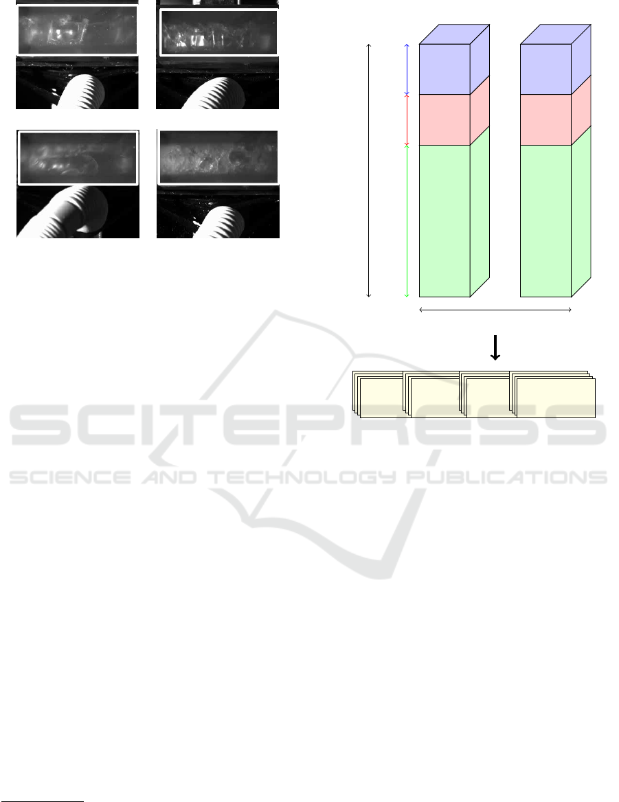
Figure 1: Liquid-gas flow visualization with the rotation ve-
locities of (a) 200 rpm, (b) 300 rpm, (c) 400 rpm, and (d)
500 rpm.
automobile engine. The dataset contains 18 grayscale
video clips (30 fps) and each clip has a duration of
about 10 to 15 minutes. There are 9 classes, corre-
sponding to the simulated rotation velocities of the
engine. Each class is represented by two videos. In
Figure 1, the movement of the liquid (glycerine) is
shown for motor speeds of 200, 300, 400 and 500
rpm. For our experiments, the only interesting area
in each video is the textures of the fluid inside the
gallery. The tube and the surroundings should not be
taken into account.
In order to extract the interesting areas in the
videos, we used a traditional tracking method which
is called ’Boosting’ (Grabner et al., 2006). This al-
gorithm is originally used for face tracking using a
Haar cascade-based face detector. In the first frame of
each video, we manually draw a bounding box around
the interesting area. Then, this box is tracked and ex-
tracted in the rest of the video (see Figure 3).
Dataset Structure. Our dataset contains 9 motor
speed classes and each class contains 2 videos of 30
fps which last about 10 to 15 minutes. We downsam-
ple it in time by a factor of 3, and divide each video
into sequences of 30 consecutive frames without over-
lapping. This gives us a dataset
1
with around 6000
sequences of 30 consecutive frames. The dataset is
split as follows: the first 60 percents of each video
sequence are for training, the next 20% are for vali-
dation and the remaining (20% of the video) are for
testing. Figure 2 shows the way how we divide our
1
Due to the large size of the dataset (about 24Gb), only
the corresponding downsampled and cropped videos which
contain only fluids textures are available at https://gitlab.
com/lphatnguyen/automobile-engine-rotation-velocity.
Video 1 Video 2
Class c
Train Validation
Test
Video of L frames
Sequence of
30 frames
Sequence of
30 frames
Sequence of
30 frames
Sequence of
30 frames
Figure 2: Dataset structure.
data. In the training process, we use the validation
set to select the parameters giving the best accuracy.
These parameters are then used for the test test.
4 CLASSIFICATION OF
COOLING GALLERY VIDEO
SEQUENCES
In this work, we compare two methods for our classi-
fication task:
• A method based on dense trajectories, optical flow
and a SVM classifier.
• A deep network based on spatial and temporal
convolutions.
4.1 Dense Trajectories
A first approach to classify two-phase flow videos is
to track liquid particles and to model explicitly trajec-
tories of interest points inside each video sequence of
30 frames. Indeed, modeling such trajectories could
help engineers to analyze the fluid movements and
Trajectory Extraction and Deep Features for Classification of Liquid-gas Flow under the Context of Forced Oscillation
19
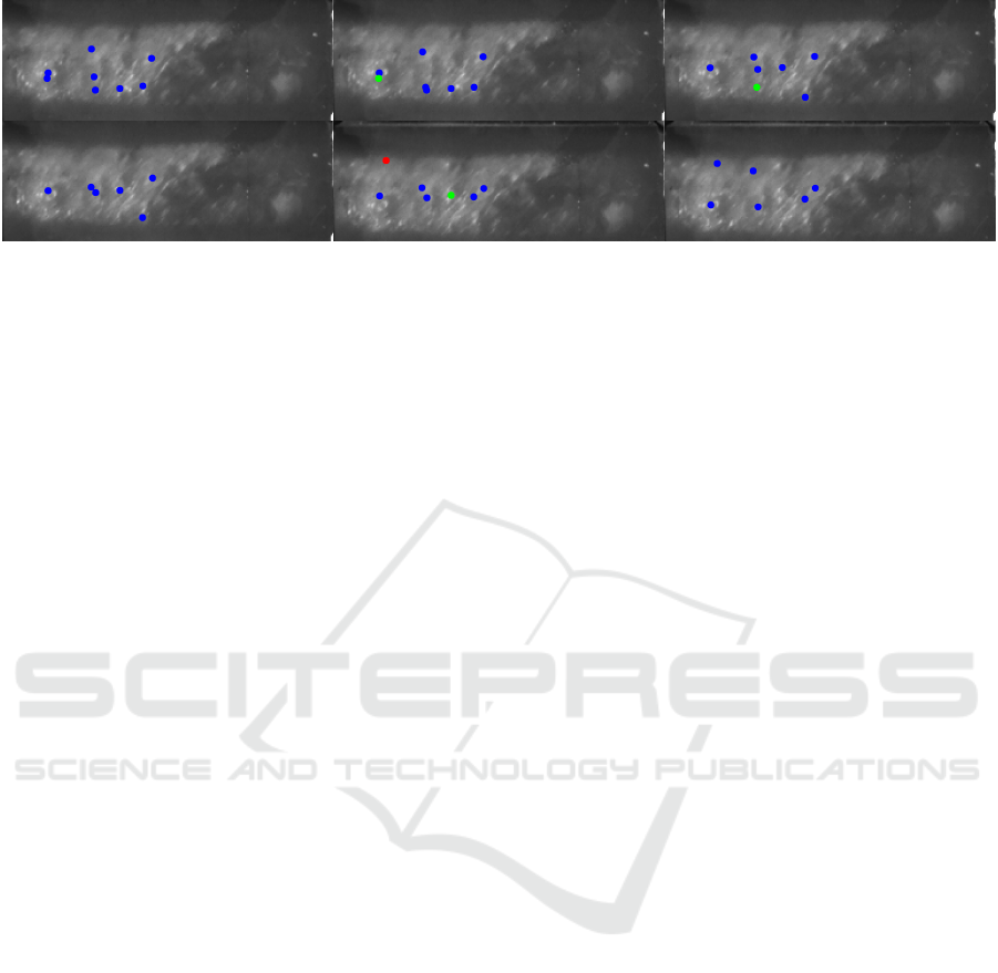
Figure 3: Dense sampled points are tracked using the dense sampling method in (Wang et al., 2013). In this sequence of 6
frames (from left to right over two lines), if a new point is detected, it is colored in red; if the point is tracked in the next frame
and the trajectory has not ended yet, the tracked point is in blue otherwise the last point of the trajectory is colored in green.
its behaviour. This is the straight forward approach
towards the final goal of the application domaine of
this study. Among many traditional trajectory extrac-
tion algorithms, the method proposed by (Wang et al.,
2013) has shown its effectiveness. In (Wang et al.,
2013), keypoints are detected using a dense sampling
method. These keypoints are then tracked in the fol-
lowing frames inside dense cubes along the trajectory.
These cubes are subdivided by a spatio-temporal grid
of size n
τ
×n
σ
×n
σ
. Features are extracted from these
dense cubes to model each trajectory. These ones are
clustered to generate Bag-of-Features, and then clas-
sification is performed using a SVM model.
The details of the approach is given here. First of
all, points are sampled on a grid spaced by w pixels
on a starting frame at multiple scales like in (Wang
et al., 2013). However, all points on the grid cannot
be tracked so these points are selected by using the
criterion of (Jianbo Shi and Tomasi, 1994). This cri-
terion helps to remove selected points if the eigenval-
ues of the auto-correlation matrix are too small. The
threshold T used is the same as in (Wang et al., 2013):
T = 0.001 × max
(x,y)∈I
(min(λ
1
(x, y), λ
2
(x, y))) (1)
where λ
j
(x, y) is the j
th
eigenvalue of the auto-
correlation matrix around the pixel (x, y). This
method can be seen as an extension of the classical
corner detection method.
Next, points are tracked to obtain trajectories, by
means of a dense optical flow field, using Farneb
¨
ack
algorithm (Farneb
¨
ack and Farneb, 2003). Further-
more, for a given tracked point, its new position is
smoothed using a median filter of size 3 ×3. Me-
dian filter is used instead of bilinear interpolation
(Wang et al., 2013) since it helps keeping sharp mo-
tion boundaries, especially in some locations such as
borders. Here, one can notice that around 60 trajec-
tories are extracted inside each video sequence (this
may vary a lot depending on the sequence).
In order to describe a trajectory, represented by its
dense cube, we use Histogram of Oriented Gradient
(HOG) (Dalal and Triggs, 2005), Histogram of Op-
tical Flow (HOF) (Laptev et al., 2008) and Motion
Boundary Histogram (MBH) (Dalal et al., 2006) as
motion and structure descriptors. HOG constructs the
distribution of directions of oriented gradients, HOF
calculates the histogram of directions of optical flows
while MBH is actually the HOG applied to dense op-
tical flow images.
Moreover, normalized displacement vector mag-
nitudes are also used as dense trajectories features and
are added to the final feature vector describing one
trajectory.
After this step, one codebook (visual dictionary)
is computed for each of the 5 types of trajectory fea-
ture vector (dense trajectories, HOG, HOF, MBHx,
MHBy). The construction of a codebook is done by
clustering the trajectory feature vectors of all training
sequences using K-means (Figure 4). The centroids
found by K-means are the visual words used in the
codebooks, and represent typical trajectories, for the
considered feature type. We denote this visual dictio-
nary by {w
1
, ...w
M
}, where M is the chosen number
of visual words, regardless of the considered feature
type.
Then, for each video sequence of the training set,
a bag-of-features (BoF) is created (Figure 5). Since
there is an arbitrary number of trajectories within a
sequence to be classified, the BoF approach allows to
obtain a constant-size final feature vector for each se-
quence. A BoF is a histogram counting the number
of occurrences of each visual word in the codebook.
The concatenation of the histograms (of the 5 features
types) is used as the final feature vector for classifi-
cation. This final feature vector is of size 5M. When
constructing an histogram, each descriptor is assigned
to the closest vocabulary word w
i
using Euclidean dis-
tance. The corresponding bin is increased.
For the classification step, we use the SVM algo-
rithm with an RBF-χ
2
kernel which is applied to BoF
VISAPP 2020 - 15th International Conference on Computer Vision Theory and Applications
20
Sequence 1
Sequence 2
.
.
.
Sequence S
Keypoint detection
and feature extraction
Keypoint detection
and feature extraction
.
.
.
Keypoint detection
and feature extraction
Codebook Construction
using K-means clustering
Dense
Trajectories
Codebook
HOG
Codebook
HOF
Codebook
MBH
Codebooks
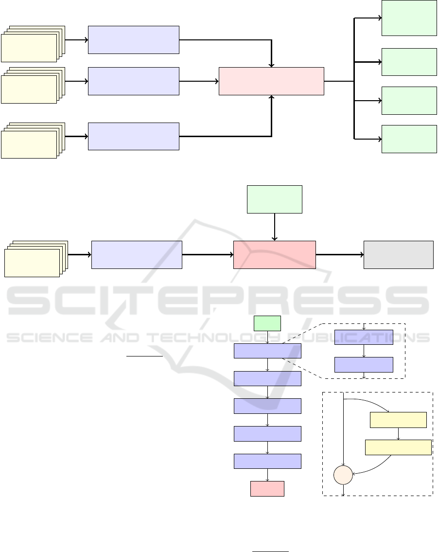
Figure 4: The construction of codebooks based on the calculated trjaectory feature vectors from video sequences.
Sequence s
Keypoint detection
and feature extraction
Constructed
codebooks
Vector quantization Bag-of-Features
Figure 5: Bag-of-features are created by encoding the trajectory feature vectors inside a sequence thanks to existing code-
books.
of sequences (Zhang et al., 2007). For two BoF vec-
tors a, b ∈R
d
, the χ
2
kernel is
K(a,b) = exp
−γ
d
∑
i=1
(a
i
−b
i
)
2
a
i
+ b
i
!
(2)
In our case, the size of the BoF vectors is d = 5M.
4.2 Deep Learning Methods
4.2.1 (2+1)D Convolution
As mentioned in section 2, R(2+1)D model has shown
its efficiency in both accuracy and size. In (Tran et al.,
2018), it is shown that a convolution in 3 dimensions
can be decomposed into a 2D spatial convolution and
a 1D temporal convolution as 2 successive steps. Let
us consider a 3D convolution layer i made of N
i
filters,
each of size N
i−1
×t ×d ×d, where t and d represent
the temporal and spatial size of the kernel respectively
and N
i−1
is the input dimension (dimension of data or
of previous layer, other than spatial and temporal, i.e.
number of channels in input images or frames). It is
decomposed into M
i
spatial filters of size N
i−1
×1 ×
d ×d and N
i
temporal filters of size M
i−1
×t ×1 ×
1. The parameter M
i
is defined as the dimension of
a subspace in which the signal is projected between
Input
R(2+1)D Block
R(2+1)D Block
R(2+1)D Block
R(2+1)D Block
R(2+1)D Block
Output
(2+1)D Conv
(2+1)D Conv
Spatial Conv
Temporal Conv
+
M
i
N
i−1
N
i
Figure 6: General architecture of R(2+1)D Convolution and
the decomposition of a 3D filters block.
spatial and temporal convolutions and is calculated as:
M
i
=
td
2
N
i
N
i−1
d
2
N
i−1
+tN
i
. A convolution of (2+1)D is similar to
the P3D-A model from (Qiu et al., 2017) but without
the bottleneck at the end of a residual layer. Figure
6 illustrates the overall architecture of the R(2+1)D
model.
Trajectory Extraction and Deep Features for Classification of Liquid-gas Flow under the Context of Forced Oscillation
21
4.2.2 Difference of Gaussian Combined with
R(2+1)D
In our study, we also propose to pre-process videos
before feeding the R(2+1)D network. Indeed, in our
opinion, dynamic textures in our dataset are very dif-
ficult and the process should focus on important inter-
est points, as for dense trajectory method. The multi-
scale Laplacian-of-Gaussian (LoG) pyramid is at the
basis of many successful keypoint extraction meth-
ods, such as SIFT (Lowe, 2004). In our context, we
draw inspiration from it in order to select visually in-
teresting parts of the liquid movement. Salient liquid
particles appear as specularities, making bright blobs
surrounded by darker pixels, which can be detected
using the LoG function. We made the hypothesis that
using these differences of Gaussian on multiple scales
would help the deep learning model.
As in (Lowe, 2004), the LoG is approximated by
the Difference of Gaussian for each pair of successive
scales as:
DoG(x, y)
i
= L(x, y; σ
i
) −L(x, y;σ
i−1
) (3)
where L(·;σ
i
) is the convolution of input image with a
2D Gaussian of standard-deviation σ
i
. Scales follow a
geometric sequence, σ
i
= ησ
i−1
, with initial scale σ
1
and scale factor η.
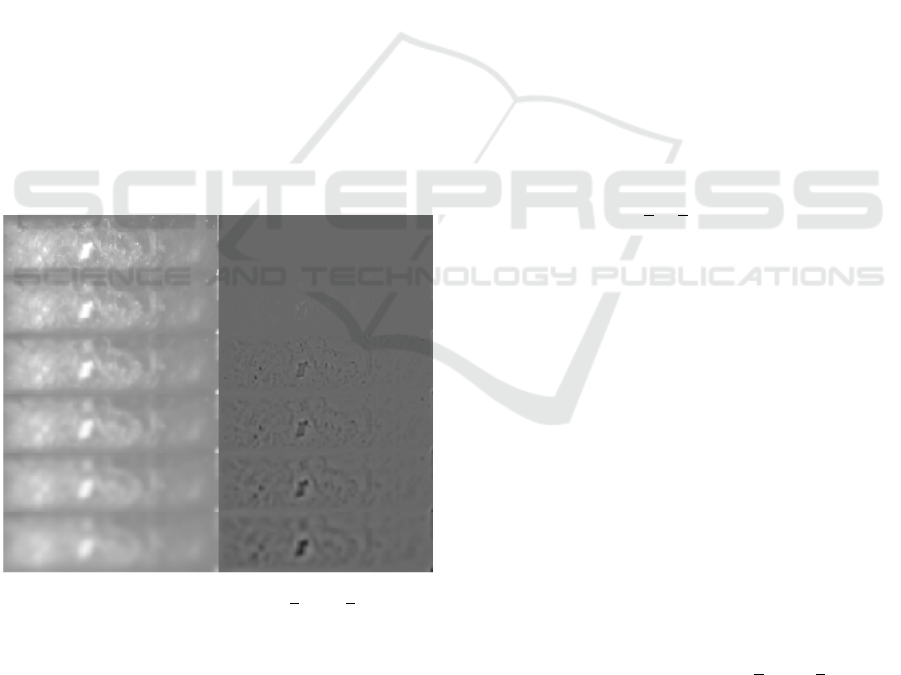
Figure 7: DoG images of a frame at motor speed of 600
rpm with F = 5 different scales: {1,
√
2, 2, 2
√
2, 4}. First
row contains only original frame. In the second row, the
first column contains blurred images of the original frame
on different scales; the second column contains the DoG
for each pair of successive scales.
Figure 7 shows the successively smoothed im-
ages L(·, σ
i
) (left column) and corresponding DoG(·)
i
(right column). In the DoG images, interesting spec-
ularities of liquid particles have negative values, ap-
pearing as dark pixels. We believe that the spatio-
temporal textures, created by the motion of these
specularities, are the main visual cues to extract, in or-
der to classify the motion speed. Hence, we integrate
this prior into our deep network: instead of taking the
initial grayscale frames as inputs, we feed the network
with a thresholded negative multiscale DoG pyramid.
Every pixel (x , y) for which −DoG(x, y)
i
< 0 is set
to 0 (Figure 8). The number of scale factors F is con-
sidered as the number of channels, so that the input
of the network is a L ×F ×H ×W tensor, where L is
the number of frames in a sequence; F is the number
of scales; H and W are the height and width of the
original frame.
5 EXPERIMENTS
In this section, we present an evaluation of the two
different methods. The accuracy corresponds to the
average of the classification rates for each class (one
should remind that a given class corresponds to a fixed
motor speed).
5.1 Experimental Setup
Dense Trajectories. In this method, we keep the
default parameters from (Wang et al., 2013). We use
3 spatial scales {1,
√
2,
√
3}, creating 3 spatial levels
for each frame. The size of the median filter is fixed
to 3 ×3 . Furthermore, the length of trajectories L
(inside sample sequences of 30 frames) is fixed to
15 frames. The cube volume in which a trajectory
is extracted is L ×N ×N with L = 15 and N = 32.
The volume is subdivided into a spatio-temporal
grid of size n
τ
×n
σ
×n
σ
with n
τ
= 3, n
σ
= 2. The
number of visual word per feature type is analyzed
to find out the optimal M
opt
for each feature type
or their combination. In our experiment, we study
M ∈ {1000, 1500, . . . , 6500, 7000}.
R(2+1)D Network. The R(2+1)D convolutional
network takes sequences of 30 frames with a size
of 96 ×256 as input. In this section, we report the
results with two kinds of inputs: original sequences
of grayscale frames and sequences of DoG frames
extracted from original data as explained in section
4.2.2. The sequences of DoG images have 5 channels,
corresponding to the 5 scales {1,
√
2, 2, 2
√
2, 4}.
Training and Evaluation. During the training pro-
cess, other parameters that have not been already fixed
are varied and we validate the performance on the val-
idation set to keep the best ones. We then use these
parameters to compute the final results on the test set.
VISAPP 2020 - 15th International Conference on Computer Vision Theory and Applications
22
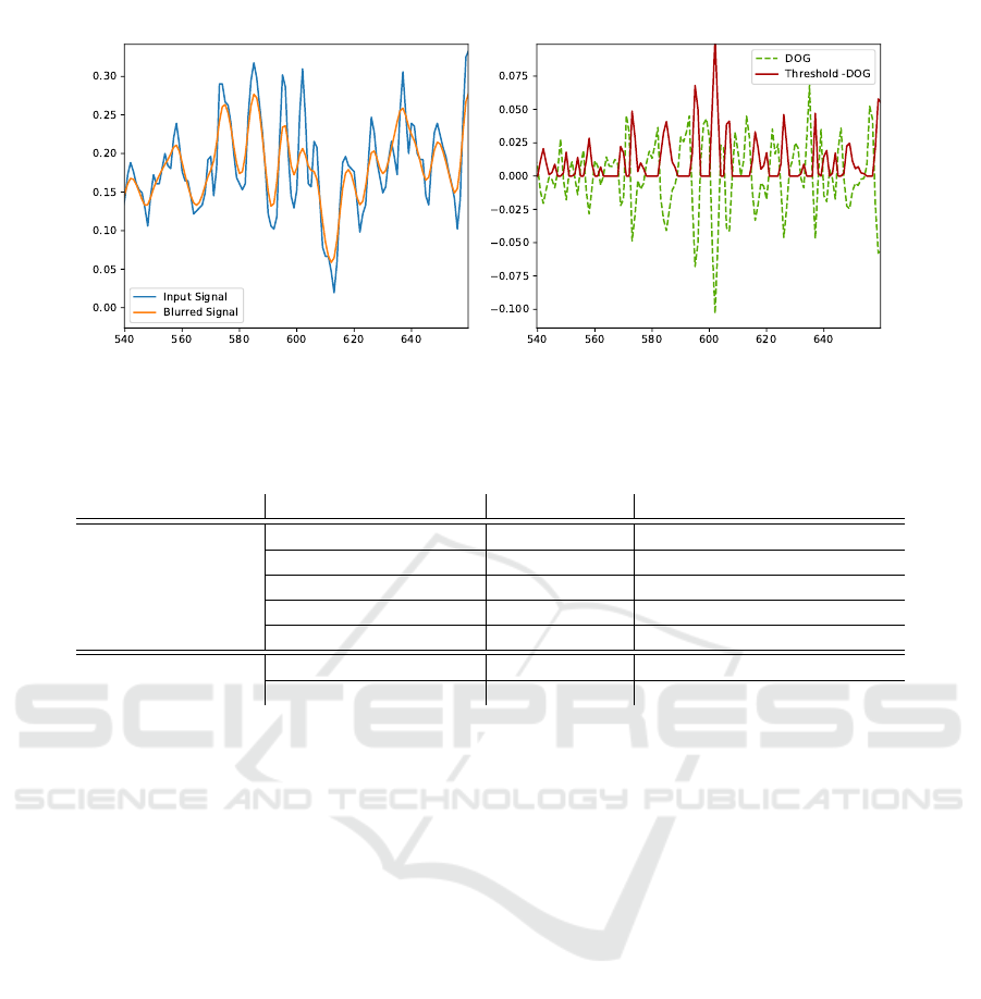
Figure 8: A toy example of the DoG on a 1D signal as pre-processing method before the neural network model.
Table 1: Performance comparison of the different approaches studied on our dataset of liquid-flow videos. The model R(2+1)D
with DoG pre-processing outperforms other techniques. The last two columns indicate the accuracy of each method and its
average execution time for each clip of 30 frames in the test set. ‘–’: Not available.
Methods Accuracy (%) Avg. exe. time per clip (ms)
Dense Trajectories
Displacements 27.74 –
HOG 54.12 –
HOF 24.73 –
MBH 50.00 –
Combined features 59.06 –
R(2+1)D
Grayscale Frames 78.06 9
DoG Frames(5 scales) 81.39 11
For the neural network approach, the training is fixed
to 50 epochs. The batch size in the training process is
4, and the ADAM algorithm is used as the optimizer
at a fixed learning rate of 10
−3
. For the dense trajec-
tories method, the codebook of each descriptor is con-
structed with M visual words. As for the SVM model,
we analyze the performance of the model by varying
the penalty parameter C (from 5.0 to 50.0 with a step
of 5.0) and the kernel coefficient γ (from 0.01 to 0.5
with a step of 0.01). The parameters which give the
best performance on the validation set are selected for
the test set. The best results on each feature type or
their combination are shown on Table 1.
All the scripts of our experiments are written in
Python. We use Pytorch as a framework and the train-
ing of the neural network is done on different types of
GPU. For the training (R(2+1)D+DOG), a NVIDIA
Tesla K80 is used and NVIDIA Tesla P100 for the
training of only grayscale frames. For the testing
phase, we only use the Tesla K80 for the evaluation
of the trained models. As for the dense trajectories
method, the an Intel i7 is used for the whole process.
5.2 Experimental Results
The aim of our experiments is to evaluate the corre-
lation between motor speeds and fluids dynamic tex-
tures in the cooling gallery in terms of video classi-
fication, as a first step before flow patterns and tra-
jectory analysis. For the dense trajectory method, we
compare the accuracy by using each individual fea-
ture and their combination.
Table 1 illustrates the results obtained by all the
methods. As expected, deep learning based meth-
ods outperform the hand-crafted features method by
at least 20%. Moreover, when comparing the two
R(2+1)D based methods, the network with the pre-
processed inputs with DoG gives a better result by
almost 3%. This shows the interest of the pre-
processing step for such kind of complex spatio-
temporal texture analysis. Nevertheless, one should
note that such kind of pre-processing to focus on spec-
ularities is not compatible with dense trajectories ex-
traction. Indeed, performing such experiments, the
accuracy is lower than the one of classical trajectory
model, more probably because the number of key-
points extracted from this specularity representation
is too small to extract relevant trajectories (this is what
we observed).
Trajectory Extraction and Deep Features for Classification of Liquid-gas Flow under the Context of Forced Oscillation
23
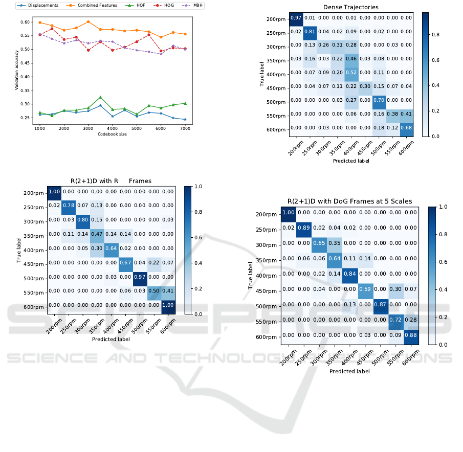
Figure 9: An analysis of the impact of codebook sizes on
the accuracy on the validation set.
aw
Figure 10: Confusion matrix of R(2+1)D on raw grayscale
frames.
An analysis of the impact of codebook size is
shown in Figure 9. The validation set is used in order
to find out the optimal codebook size for each type of
feature vector. As shown in this figure, displacement
and HOF features show their weakness in classifying
the rotation velocity videos. The highest obtained ac-
curacy is found at the codebook size of 3500 (which
are always below 35%). However, when looking at
the other feature types (HOG, MBH and combination
of these features), it can be recognized that their ac-
curacy on the validation set is much higher than the
other two features. Individually, the combination of
features always shows its superiority and its high-
est accuracy at the codebook size of 1000 and 3000
(around 60% of accuracy). The HOG feature reaches
its peak using 1500 visual words (57.58%) and the
MBH feature has 55.62% of accuracy at 1000 visual
words on the validation set.
Figure 10 shows the normalized confusion ma-
trix of R(2+1)D convolution network using only raw
grayscale frames as inputs. We note that the model
classifies well the sequences corresponding to mo-
Figure 11: Confusion matrix of dense trajectories method.
Figure 12: Confusion matrix of R(2+1)D on DoG frames.
tor speeds of 200, 300, 500 and 600 rpm (more than
80%). Particularly, the model classifies well 100% of
sequences with the motor speeds of 200 and 600 rpm
and 90% for the class of 500 rpm. In Figure 12, the
confusion matrix of R(2+1)D convolution network
combined with DoG features is shown. The model
classifies perfectly the data from the class 200 rpm
(100%) and pretty well with some other classes like
250, 400, 500 and 600 rpm (around 90% of accuracy).
We can also see that the results of this model are
distributed more equally than the model without the
pre-processing step (59%-100% compared with 47%-
100%). Considering, the dense trajectory method
(Figure 11), it can only classify well the first class
200 rpm (96%) and somehow not bad the classes of
250 rpm and 600 rpm (72% and 71% respectively).
From these experimental results, the deep
learning-based methods again show theirs efficiency
on dynamic texture classification task over hand-
crafted features. This may be due to two reasons.
VISAPP 2020 - 15th International Conference on Computer Vision Theory and Applications
24

Firstly, contrarily to our hypotheses, dense trajecto-
ries are probably not the right way to describe dy-
namic textures for such kind of liquid movements.
Secondly, the extraction of such trajectories is pos-
sibly not good enough with state-of-the-art approach
and then it should be adapted. It could be for exam-
ple because of the fixed trajectory length. Indeed, we
may lose some trajectories that have length shorter or
longer than 15 frames and therefore a lot of interest-
ing spatio-temporal information may be lost during
the tracking process. This might be particularly true
in our case when the two phases of the mechanical
process are creating droplets and bubbles.
6 CONCLUSIONS
In this paper, a new dataset based on two-phased flow
visualization inside a simulation of a cooling gallery
is proposed to the community. This dataset opens a
field for research on dynamic texture analysis and es-
pecially for flow patterns extraction and analysis of
their trajectories. Here, flow patterns are used for
a classification task: two classical computer vision
techniques are studied in order to validate the fact that
there exists a correlation between the motor speed and
the movements of fluids in a two-phase flow engineer-
ing process. The first approach, based on the state-of-
the-art approach to extract and characterize trajecto-
ries, seems not to work well on fluids particles even
if there exists room for improvements. This repre-
sents a first challenging task since being able to ex-
tract and analyze these trajectories is really important
for the considered application domain: being able to
analyze and describe the behaviour of particules and
thus their trajectories could be useful for engineers.
On the other side, deep learning approaches based on
R(2+1)D convolutions give better results even if not
completely satisfying. Consequently, we propose in
this study to improve the approach adding a prepro-
cessing step that changes the original videos repre-
sentation to highlight specularities of fluids, thanks to
DoG. The counterpart of this deep method is the loss
of explanability of the decision and modeling process.
Then, another challenging task brought by this study
is how to use deep features to extract flow patterns and
their trajectories to make further analysis possible.
ACKNOWLEDGEMENTS
This work was supported by University of Zhejiang
and Haoyi Niu in particular. We gratefully acknowl-
edged the support of his work with the video data used
for this research.
REFERENCES
Andrearczyk, V. and Whelan, P. F. (2018). Convolu-
tional neural network on three orthogonal planes for
dynamic texture classification. Pattern Recognition,
76:36–49.
Crivelli, T., Cernuschi-Frias, B., Bouthemy, P., and Yao,
J.-F. (2013). Motion Textures: Modeling, Classifi-
cation, and Segmentation Using Mixed-State Markov
Random Fields. SIAM Journal on Imaging Sciences,
6(4):2484–2520.
Dalal, N. and Triggs, B. (2005). Histograms of Ori-
ented Gradients for Human Detection. In 2005 IEEE
Computer Society Conference on Computer Vision
and Pattern Recognition (CVPR’05) , volume 1, pages
886–893. IEEE.
Dalal, N., Triggs, B., Schmid, C., Dalal, N., Triggs, B.,
Schmid, C., Detection, H., and Oriented, U. (2006).
Human Detection Using Oriented Histograms of Flow
and Appearance. European Conference on Computer
Vision (ECCV), 1(1):428–441.
Farneb
¨
ack, G. and Farneb, G. (2003). Two-Frame Motion
Estimation Based on. Lecture Notes in Computer Sci-
ence, 2003(1):363–370.
Grabner, H., Grabner, M., and Bischof, H. (2006). Real-
Time Tracking via On-line Boosting. In Procedings
of the British Machine Vision Conference 2006, pages
6.1–6.10. British Machine Vision Association.
Jansson, Y. and Lindeberg, T. (2018). Dynamic Texture
Recognition Using Time-Causal and Time-Recursive
Spatio-Temporal Receptive Fields. Journal of Mathe-
matical Imaging and Vision, 60(9):1369–1398.
Jianbo Shi and Tomasi (1994). Good features to track.
In Proceedings of IEEE Conference on Computer Vi-
sion and Pattern Recognition CVPR-94, volume 169,
pages 593–600. IEEE Comput. Soc. Press.
Krizhevsky, A., Sutskever, I., and Hinton, G. E. (2017). Im-
ageNet classification with deep convolutional neural
networks. Communications of the ACM, 60(6):84–90.
Laptev, I., Marszalek, M., Schmid, C., and Rozenfeld,
B. (2008). Learning realistic human actions from
movies. In 2008 IEEE Conference on Computer Vi-
sion and Pattern Recognition, pages 1–8. IEEE.
Lowe, D. G. (2004). Distinctive image features from scale-
invariant keypoints. International Journal of Com-
puter Vision, 60(2):91–110.
Lu, Z., Xie, W., Pei, J., and Huang, J. J. (2007). Dynamic
texture recognition by spatio-temporal multiresolution
Histograms. Proceedings - IEEE Workshop on Motion
and Video Computing, MOTION 2005, (200338):241–
246.
Nelson, R. C. and Polana, R. (1992). Qualitative recogni-
tion of motion using temporal texture. CVGIP: Image
Understanding, 56(1):78–89.
Qi, X., Li, C. G., Zhao, G., Hong, X., and Pietik
¨
ainen, M.
(2016). Dynamic texture and scene classification by
transferring deep image features. Neurocomputing.
Trajectory Extraction and Deep Features for Classification of Liquid-gas Flow under the Context of Forced Oscillation
25

Qiu, Z., Yao, T., and Mei, T. (2017). Learning Spatio-
Temporal Representation with Pseudo-3D Residual
Networks. Proceedings of the IEEE International
Conference on Computer Vision, 2017-Octob:5534–
5542.
Renaud, P. and Chetverikov, D. (2005). Using Normal Flow
and Texture Regularity. Pattern Recognition and Im-
age Analysis, (June 2005):223–230.
Tran, D., Bourdev, L., Fergus, R., Torresani, L., and Paluri,
M. (2015). Learning spatiotemporal features with 3D
convolutional networks. Technical report, Santiago.
Tran, D., Wang, H., Torresani, L., Ray, J., LeCun, Y., and
Paluri, M. (2018). A Closer Look at Spatiotempo-
ral Convolutions for Action Recognition. In 2018
IEEE/CVF Conference on Computer Vision and Pat-
tern Recognition, pages 6450–6459. IEEE.
Wang, H., Kl
¨
aser, A., Schmid, C., and Liu, C.-L. (2013).
Dense Trajectories and Motion Boundary Descrip-
tors for Action Recognition. International Journal of
Computer Vision.
Zhang, J., Marszałek, M., Lazebnik, S., and Schmid, C.
(2007). Local features and kernels for classification of
texture and object categories: A comprehensive study.
International Journal of Computer Vision, 73(2):213–
238.
VISAPP 2020 - 15th International Conference on Computer Vision Theory and Applications
26
