A Hybrid Approach for Segmenting and Fitting Solid Primitives to 3D

Point Clouds

Markus Friedrich

, Steffen Illium

, Pierre-Alain Fayolle

and Claudia Linnhoff-Popien

Institute for Computer Science, LMU Munich, Oettingenstraße 67, Munich, Germany

The University of Aizu, Ikki machi, Aizu-Wakamatsu, Japan

Keywords:

3D Computer Vision, Deep Learning, Evolutionary Computing, Fitting, RANSAC, Segmentation.

Abstract:

The segmentation and ﬁtting of solid primitives to 3D point clouds is a complex task. Existing systems are

restricted either in the number of input points or the supported primitive types. This paper proposes a hybrid

pipeline that is able to reconstruct spheres, bounded cylinders and rectangular cuboids on large point sets. It

uses a combination of deep learning and classical RANSAC for primitive ﬁtting, a DBSCAN-based clustering

scheme for increased stability and a specialized Genetic Algorithm for robust cuboid extraction. In a detailed

evaluation, its performance metrics are discussed and resulting solid primitive sets are visualized. The paper

concludes with a discussion of the approach’s limitations.

1 INTRODUCTION

The reconstruction of geometric primitives from 3D

point clouds is important in quality assurance and re-

verse engineering of mechanical structures and plays

a key-role for a lot of computer aided design mod-

elling tasks. Building a robust primitive reconstruc-

tion pipeline is complex: It needs to account for noise

in the input point cloud, ﬁnd all potential primitives

and estimate their parameters as precisely as possible.

We propose a hybrid pipeline for the robust seg-

mentation and ﬁtting of solid primitives that combines

the strengths of multiple approaches with a new tech-

nique for rectangular cuboid (or simply cuboid) gen-

eration based on Evolutionary Computing. A deep

neural network is adapted and trained to label points

from a point cloud with associated primitive types

(cylinder, sphere, plane). Then, the point cloud is

clustered based on point coordinate, surface normal

and primitive type label. A classic approach (efﬁcient

RANSAC (Schnabel et al., 2007)) for primitive ﬁtting

is applied to each cluster. Since the primitive ﬁtting

step does not generate closed solids, we introduce an

additional step that estimates the height of cylinders

and generates cuboids based on ﬁtted planes using a

Genetic Algorithm (GA).

The paper makes the following contributions:

• A modiﬁed deep neural network for primitive type

detection together with a fast training data set gen-

erator and a partitioning scheme for better scala-

bility with respect to input point cloud size.

• An improved primitive ﬁtting method that uses

density-based clustering to stabilize the stochastic

ﬁtting process and to decrease parameter sensitiv-

ity.

• A cuboid generation scheme based on a GA that

assembles ﬁtted planes to form cuboids.

• A full pipeline for the segmentation and ﬁtting

of solid primitives that combines state-of-the-art

techniques with the aforementioned, newly devel-

oped components.

The rest of the paper is structured as follows: We re-

view related works in Section 2. Section 3 describes

the tools that we use, followed by our proposed seg-

mentation and ﬁtting pipeline in Section 4. The eval-

uation (Section 5) discusses experimental results and

limitations. A conclusion together with future work is

given in Section 6.

2 RELATED WORK

Segmentation, primitive detection and primitive ﬁt-

ting are well studied problems in computer graphics,

computer aided design and related engineering disci-

plines. Several solutions have been proposed over the

years. In the following, we list some of the most rele-

Friedrich, M., Illium, S., Fayolle, P. and Linnhoff-Popien, C.

A Hybrid Approach for Segmenting and Fitting Solid Primitives to 3D Point Clouds.

DOI: 10.5220/0008870600380048

In Proceedings of the 15th International Joint Conference on Computer Vision, Imaging and Computer Graphics Theory and Applications (VISIGRAPP 2020) - Volume 1: GRAPP, pages

38-48

ISBN: 978-989-758-402-2; ISSN: 2184-4321

vant works. The reader is also referred to the surveys

on mesh segmentation (Shamir, 2008) and primitive

detection (Kaiser et al., 2019) for a broader overview

of existing works.

2.1 Geometric Approaches

Segmentation, primitive detection and ﬁtting are

some of the necessary steps in reverse engineering of

3D data, which is the process of recovering a com-

puter model of a 3D shape from acquired data. See,

for example, (V

arady et al., 1998; Marshall et al.,

2001; Benk

o et al., 2001) and the references therein.

More recently, these problems of segmentation

and primitive detection have gained interest in the

computer graphics community. Some of the works

are only concerned with the segmentation of the input

point cloud (or triangle mesh) and assigning a prim-

itive type (e.g. cylinder, plane, torus) to each clus-

ter as, for example, in (Cohen-Steiner et al., 2004;

Lavou

e et al., 2005).

For other applications, it is also necessary to re-

cover the parameters (e.g. the radius and center of a

sphere) deﬁning the primitives (Vanco and Brunnett,

2004; Attene et al., 2006; Schnabel et al., 2007; Li

et al., 2011; Le and Duan, 2017) in addition to the

segmentation and assignment of a primitive type to

each point.

A popular family of approaches relies on

RANSAC (Fischler and Bolles, 1981) and its vari-

ants. The efﬁcient RANSAC method (Schnabel et al.,

2007) is a very fast RANSAC-based approach for

detecting primitives of different types in a 3D point

cloud, and recovering the corresponding parameters.

This approach is improved in (Li et al., 2011) by en-

forcing additional constraints during the ﬁtting pro-

cess (e.g. parallelism of the cylinders’ main axes).

There are two differences between these approaches

and ours: First, we apply RANSAC to a pre-clustered

(by primitive type) point cloud, which allows us to

limit the primitives to try and make the process more

robust and less parameter sensitive. Second, unlike

RANSAC that ﬁts unbounded primitives (planes, un-

bounded cylinders, . . . ), we generate bounded prim-

itives, in particular planes that are combined into

cuboids.

In some application domains, additional con-

straints are imposed on the primitives in considera-

tion. For example, in the reconstruction of buildings

from 3D point clouds, only planes need to be detected

and ﬁtted, see e.g. (Monszpart et al., 2015; Oesau

et al., 2016). These planes are then combined to form

cuboids (Xiao and Furukawa, 2014; Li et al., 2016)

or more complex polyhedral shapes (Nan and Wonka,

2017). Contrary to these approaches, our method is

not limited to cuboids. Additionally, we have no lim-

itations, such as, all planes are required to be orthog-

onal to the main axes.

2.2 Machine Learning Approaches

With the increase of available 3D data sets, learn-

ing based approaches have gained interest as possible

techniques for primitive detection and ﬁtting.

Earlier works, such as (Kalogerakis et al., 2010;

Kim et al., 2013), are based on traditional machine

learning techniques for learning segmentation and la-

belling (Kalogerakis et al., 2010) or template shapes

corresponding to each part (Kim et al., 2013).

Most of the recent approaches are based on deep

learning, however. Segmentation of point clouds us-

ing deep learning is proposed in the PointNet (Qi

et al., 2017a) and PointNet++ (Qi et al., 2017b) pa-

pers.

In (Li et al., 2019), Li et al. propose an end-to-end

learning framework for segmenting, detecting and ﬁt-

ting primitives (plane, sphere, cylinder and cone) in

3D point clouds. It is interesting to note that this

approach relies on the point coordinates only, while

most methods (including the more classic and geo-

metric approaches) usually assume as well the pres-

ence of the surface normal at each point in the in-

put point cloud. Other approaches, such as (Zou

et al., 2017; Tulsiani et al., 2017), try to approxi-

mate the input 3D shape by predicting a collection

of cuboids. The approach described in (Paschalidou

et al., 2019) extends the previous works by replac-

ing cuboid primitives with superquadric primitives.

Generalizing these primitives leads to the learning of

shape templates (Genova et al., 2019). Compared to

these approaches, our method is not limited to a single

primitive type (e.g. cuboids). Additionally, there is no

restriction on the size of the input point cloud, which

these deep learning-based methods usually have.

3 BACKGROUND

In this section, we give a brief description of the tools

that are used in our approach described in Section 4.

3.1 Farthest Point Sampling

Farthest Point Sampling (FPS) is used as in (Qi et al.,

2017a) to down-sample a point cloud to k points while

still covering a certain surface area uniformly. It is

based on the idea of iteratively selecting the next sam-

ple as the farthest away point from the set of points

A Hybrid Approach for Segmenting and Fitting Solid Primitives to 3D Point Clouds

selected so far. We use a greedy implementation with

a O (n

) computational complexity (n is the number

of points in the point cloud to be down-sampled) that

meets our requirements in terms of point cloud size

and running time.

3.2 DBSCAN

Density Based Spatial Clustering of Applications

with Noise (DBSCAN) is a popular clustering method

introduced in (Ester et al., 1996). It works by start-

ing from high density samples and expanding clusters

from these samples. This expansion is done by con-

sidering the samples in the neighborhood. Neighbors

are determined based on a given metric. We use DB-

SCAN for clustering neighbor points assigned to the

same primitive type (Section 4.2). In (Czerniawski

et al., 2018), DBSCAN is also used for point cloud

clustering but without an additional per-point primi-

tive type label like in this work.

3.3 PointNet++

PointNet (Qi et al., 2017a) and its successor

PointNet++ (Qi et al., 2017b) are deep neural net-

works specialized in the processing of point clouds

(semantic segmentation, classiﬁcation). PointNet++

offers better generalization capabilities and robust-

ness than PointNet by learning the context of local

features. We use a variant of PointNet++ for assign-

ing a label (primitive type) to each point in the input

point cloud (Section 4.2).

3.4 RANSAC

RANSAC (Fischler and Bolles, 1981) is a method for

estimating the parameters of a model (e.g. the param-

eters deﬁning a plane) from a noisy data set. It works

by selecting a few points and directly determining the

parameters of the corresponding primitive. Then, all

points that are located on or near the ﬁtted primitive’s

surface are collected. The process is repeated until the

probability that the ﬁtted primitive best describes the

point cloud is above some threshold.

A RANSAC-based approach is used in our

pipeline for ﬁtting the primitives’ parameters given

computed clusters of points (see Section 4.3). We

use the efﬁcient RANSAC approach (Schnabel et al.,

2007).

3.5 Genetic Algorithms

Genetic Algorithms (GA) are biology-inspired,

stochastic metaheuristics for solving optimization

problems. The optimization process of the GA starts

with a randomly initialized population of individuals

sampled from the problem’s search space. At each it-

eration, these individuals are ranked according to their

ﬁtness score, obtained by evaluating a ﬁtness func-

tion. The best creatures are selected to be the next

generation’s parents. The parents are then recom-

bined by crossover and mutated to create offspring.

The new population is ﬁlled with the offspring to-

gether with selected surviving individuals from the

current population. This procedure is repeated until

a certain termination criteria is met. We use a GA for

combining ﬁtted planes to cuboids (Section 4.4).

3.6 Signed Distance Functions

In this work, we represent primitives using the signed

distance function to their boundary. For a solid S,

its boundary surface ∂S is implicitly deﬁned by the

zero level-set of its corresponding distance function

: {x ∈ R

: d

(x) = 0}. The surface normal at

point x ∈ R

is given by the gradient of the distance

function ∇d

(x), which has unit norm |∇d

(x)| = 1.

In this work, we consider the following primitives:

cuboids, spheres and cylinders.

4 CONCEPT

4.1 Pipeline

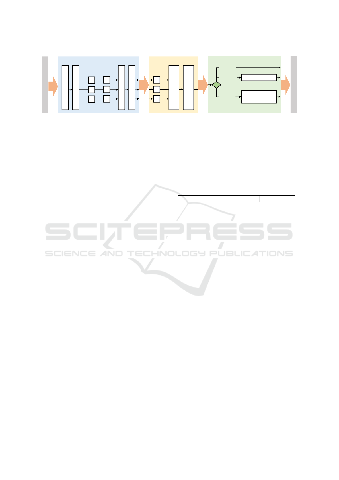
Our approach is summarized by the pipeline in Fig. 1.

It contains three major parts: The ﬁrst part primitive

type detection predicts a primitive type label (plane,

sphere, cylinder) for each point in the input point

cloud O and clusters points using DBSCAN resulting

in homogeneous clusters of points associated to prim-

itives of the same type. The clustering leads to more

stable results in the next part, the primitive ﬁtting,

which uses the efﬁcient RANSAC algorithm (Schn-

abel et al., 2007) to extract primitive parameters for

primitives in each cluster. Resulting cylinders are not

closed (i.e. their height is not determined) and planes

need to be combined to form solids (cuboids). This

is done in the last step, the solid primitive generation

step.

GRAPP 2020 - 15th International Conference on Computer Graphics Theory and Applications

solid primitive generation

primitive type detection primitive fitting

pointcloud

solid primitive

generation GA

detection

RANSAC

spatial partitioning

FPS

pre-processing

merge

solid primitives

height estimation

merge & duplicate removal

clustering

sphere

cylinder

cuboid

per-primitive FPS

Figure 1: The pipeline for the segmentation and ﬁtting of solid primitives.

4.2 Primitive Type Detection

Pre-processing. To remove outliers from the input

point cloud, we use a simple density-based unsuper-

vised outlier detection method (Breunig et al., 2000).

Additionally, we normalize the point coordinates so

that they ﬁt into a unit cube. This assumption is used

in the primitive type detection step.

Spatial Partitioning. The input point cloud is parti-

tioned in n × n × n boxes of equal dimensions using

the point cloud’s axis-aligned bounding box (AABB)

as the initial volume to partition (we used n = 2 in

the evaluation). This is done for two reasons: Firstly,

for better generalization, the model for primitive type

label prediction is trained on model partitions. Thus,

point cloud partitions are closer to what the network

has learned, which results in better predictions. Sec-

ondly, the network architecture requires a ﬁxed maxi-

mum number of points per input point cloud (we use

2048 points). The partitioning circumvents this re-

striction for the complete input point cloud since pre-

diction is done per-partition. See Fig. 6a for results of

this step.

Sampling and Detection. Since for performance rea-

sons (both in training and prediction), the maximum

input point cloud size for the PointNet++-based detec-

tion step is set to 2048, FPS with k = 2048 is applied

to each point cloud partition. Then, primitive type la-

bel prediction is conducted on each partition, result-

ing in a label (the primitive type) for each point. For

better prediction results, we extended PointNet++ to

use not only point coordinates but also point normals

for training and prediction. See Fig. 6b for results.

Merge. All point cloud partitions are merged together

resulting in a single set of labeled points.

Clustering. The point set is now clustered using DB-

SCAN. For performance reasons, the Euclidean dis-

tance is used as the distance metric for DBSCAN.

This requires a 1-hot-encoding of the primitive type

label (e.g. a cylinder’s encoding is (1,0, 0), a sphere’s

(0, 1, 0), . . . ) per point, together with its normalized

point coordinates and normal vector. Table 1 shows

the attributes of a single point as represented during

clustering. The collection of all such points is passed

to DBSCAN for clustering. The clustering process

consists of two stages: In the ﬁrst stage, the input

point cloud is clustered using o

and o

. Then, in the

second stage, resulting clusters are clustered again us-

ing o

and o

. This 2-level hierarchical approach de-

livered the best clustering results in our experiments.

Table 1: Attributes of a single point o: Coordinates, normal

vector and 1-hot-encoded primitive type vector.

= (p

, p

) o

= (n

, n

) o

= (t

)

The approach leads to clusters containing points

with the same primitive type label. Using the point’s

normal and position additionally decreases the num-

ber of primitive types per cluster. For most of our test

models this results in a 1 : 1 ratio between primitive

types and clusters. Fig. 6c illustrates examples of re-

sults obtained by the clustering step.

4.3 Primitive Fitting

RANSAC. The RANSAC primitive ﬁtting method is

applied to each cluster separately. The input is the

sampled (using FPS) cluster point cloud. The list

of primitive types for RANSAC to consider is ex-

tracted from the cluster’s predicted primitive type la-

bels available for each point. Based on our experi-

ments, this results usually in a single primitive type

- in rare cases, however, this number could be higher.

The number of primitives to detect is reduced, as well,

by the clustering, e.g. for most planes only a single

primitive needs to be ﬁtted per cluster. Both, the re-

duced number of primitive types to consider and the

smaller amount of primitives to detect, have positive

inﬂuence on the robustness and parameter sensitivity

of the RANSAC approach.

Merge and Duplicate Removal. To make the output

of RANSAC more robust, we run it multiple times on

each cluster (3 times in our experiments), collect the

ﬁtted primitives from all the runs and merge the prim-

itives that are close. This process works as follows:

Starting from the ﬁtted primitives obtained from all

A Hybrid Approach for Segmenting and Fitting Solid Primitives to 3D Point Clouds

the runs of RANSAC, we ﬁrst form clusters of close

primitives. Then, within each cluster, we merge those

primitives. Two primitives are considered to be close

if their parameters are within a certain threshold. For

example, we consider two spheres to be close if the

distance between their centers is within some thresh-

old, and similarly for their radii. Other primitives may

also involve comparing the angles between two direc-

tions and verify that they are within some threshold.

Merging close primitives is simply done by taking the

average of their deﬁning parameters. For example,

for three close spheres, we would create a new sphere

with a radius, respectively center, equal to the average

of the three spheres radii, respectively centers.

Per-Primitive Sampling. We apply FPS (usually

with k = 100) to the point set associated to each ﬁtted

primitive. This is done in order to reduce the com-

putational effort for evaluating the objective function

(Equation 1) in the GA executed in the solid primitive

generation step.

4.4 Solid Primitive Generation

4.4.1 Spheres and Cylinders

Spheres are already bounded primitives, they don’t

need to be processed any further. For cylinders, the

height must be estimated. A simple approach is used:

Each point of the point cloud corresponding to a

cylinder is projected on its main axis. The distance

between the points that are farthest away is used as

the cylinder’s height. The downside of this method is

potentially wrong alignment to other connected prim-

itives in case of missing scan points near the neigh-

boring objects.

4.4.2 Cuboids

Cuboids are more difﬁcult to reconstruct. Please note

that we use the term cuboid as an abbreviation for

a convex polyhedron with six rectangular and pair-

wise perpendicular faces (rectangular cuboid). Since

the plane primitive’s parameters are already estimated

by RANSAC, it is possible to formulate the cuboid

construction problem as a combinatorial optimization

problem over all ﬁtted planes: Given a set of n

planes P = {p

, . . . , p

−1

}, we would like to com-

pute a cuboid set C = {c

, . . . , c

−1

} containing n

cuboids that best represents the input point cloud O

according to an objective function F(C, O) to be max-

imized. Here O contains only those points from the

input point cloud that correspond to planes. To guar-

antee that plane sets form valid cuboids, we formulate

two constraints: 1) A cuboid must consist of exactly 6

planes, 2) A cuboid must contain planes that are pair-

wise parallel. Note that a plane from P can belong to

multiple cuboids.

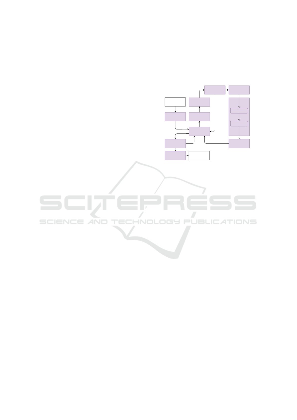
To solve this combinatorial optimization problem,

a specialized GA, depicted in Fig. 2, is used. The

details about the GA are provided below.

Variation

Population

Parents

Offspring

Crossover

Mutation

Best Individual

Selection

Initialization

Selection

Ranking

Result

Termination Check

Optimization

Ghost Plane

Generation

Figure 2: The proposed GA for solving the combinatorial

cuboid generation problem with core GA parts in purple.

Ghost Plane Generation. So-called ghost planes

are planes added to the initial set of ﬁtted planes

= P∪P

. Ghost planes are necessary in cases, such

as, where one side of a cuboid is fully covered by a

non-planar primitive (e.g. a cylinder, as depicted in

Fig. 3) Without these ghost planes, the constraint that

a plane set (cuboid) needs to have 6 planes could be

violated in the general case. Ghost planes are gener-

ated for each existing plane in P by computing the 2D

convex hull of the (projected) points associated to a

particular plane. Then, the minimum-area rectangle

that fully contains the convex hull is computed using

the Rotating Caliper Algorithm (Shamos, 1978). One

plane is generated for each side of the rectangle. Each

generated plane is perpendicular to the original plane

and fully contains the rectangle side (see Fig. 3 for

a visual explanation). Since the generation process

results in a large number of (often) similar planes,

an additional ﬁlter mechanism is applied that merges

similar planes.

Population. Each individual of the GA’s population

is a cuboid set, where each cuboid is a set of exactly 6

planes. A user-deﬁned maximum number of cuboids

C max

restricts the size of each individual.

Initialization. The population is initialized with a

set of individuals, where each individual is a cuboid

set. The cuboid set size is randomly chosen from

{1, . . . , n

C max

}. Cuboids are generated as follows: At

ﬁrst, a random plane is chosen from P

. Then, a plane

parallel to that plane is selected randomly. This is fol-

lowed by a selection of a plane that is perpendicular to

the two already selected ones. Now, a plane parallel to

GRAPP 2020 - 15th International Conference on Computer Graphics Theory and Applications

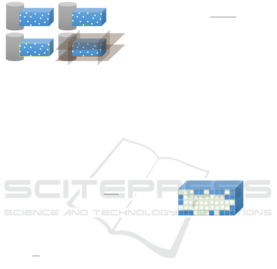
Figure 3: Ghost plane generation. Top left: The left side of

the cuboid is completely covered by the cylinder. Thus, a

plane is missing to form the complete cuboid. Ghost planes

are generated for each existing plane (the cuboid’s front

plane serves as an example). Top right: 2D convex hull,

bottom left: Minimum-area rectangle, bottom right: The 4

generated ghost planes for the cuboid’s front plane (orange).

the third plane is selected. Finally, a plane perpendic-

ular to all already selected planes is selected together

with its parallel companion. This results in a cuboid

fulﬁlling all constraints mentioned above. If a certain

selection does not lead to a valid cuboid, the process

is repeated.

Ranking. The ﬁtness function F(C, O) determines

how well a set of cuboids C (an individual in the GA)

ﬁts the point cloud O and reads:

F(C, O) = α · G(C, O) + β · A(C, O) − γ ·

|C|

C max

, (1)

where α, β and γ are weights and the last term is a

cuboid set size penalty term (|C| is the cardinality of

C). The geometry term G(C, O) counts the number

of points in the point cloud O whose distance to the

closest cuboid is below a certain ε

G(C, O) =

|O|

∑

o∈O

(

1, if min

c∈C

)| < ε

0, otherwise

(2)

where d

(·) is the signed distance function of the

cuboid c and |O| the number of points in O. Please

note that the points in O are re-projected to their corre-

sponding plane in order to account for potential noise.

The geometry term computes a score based on the

number of points in O that are close enough to the sur-

face of the closest cuboid in the cuboid set. However,

using only this metric is not enough: Even if all points

are close enough to a surface (and G(C, O) reaches its

maximum), cuboids might exist in the set that do not

contribute to the score since none of their surfaces is

the closest surface to any point. To avoid having these

additional cuboids in the set, we use two mechanisms:

First, a term to penalize large cuboid sets is used (the

third term in (1)). Second, we propose an additional

term A(C, O) that accounts for the surface area of the

cuboids that is actually covered by points of O:

A(C, O) =

∑

c∈C

|∂O

∑

c∈C

|∂c|

, (3)

where |∂O

| is the area covered by points from O as-

sociated to the surface of cuboid c and |∂c| is the sur-

face area of cuboid c.

For the area |∂O

|, an approximation is computed

using an approach based on rasterization and applied

to each of the six planes of a cuboid c. At ﬁrst, the

plane-based cuboid representation is converted to a

face-and-vertex-based representation using the Dou-

ble Description Method (Fukuda and Prodon, 1995),

resulting in 6 quads each representing a side of the

cuboid. This is needed to get a bounded area per

cuboid side. For each quad, the subset of points from

O located on or near the quad is projected onto the

quad’s 2D plane. Then, the quad is rasterized using

a raster size dependent on the density of associated

points. For each raster cell, it is checked if it contains

a point. Cells that contain a point are accumulated and

multiplied by the raster cell area to get an approxima-

tion of the surface area covered by the point subset.

See Fig. 4 for a visual description of the method for a

single quad. In order to improve performance, scores

Figure 4: The rasterization of a single cuboid side with the

covered area estimation in green.

are cached and re-used, Our tests have shown that the

cache has a hit rate of around 50%.

Selection and Variation. Two individuals are se-

lected from the population as parents using a tourna-

ment selection. The crossover operator is applied to

both parents with probability p

. It exchanges ran-

domly selected cuboid sequences (subsets with con-

tiguous indices). The mutation operator is then ap-

plied to both parents with a probability of p

. Muta-

tion comes in 4 different variants:

• New: Creates a whole new cuboid set.

• Replace: Replaces a randomly selected cuboid

with a newly created cuboid.

• Modify: Selects a cuboid randomly and ﬁnds a

new parallel plane for a randomly selected one.

• Add: Adds a randomly created cuboid to the

cuboid set.

The variant to use is chosen randomly. The selec-

tion and variation process is repeated until enough

A Hybrid Approach for Segmenting and Fitting Solid Primitives to 3D Point Clouds

offspring for the new population is generated. In ad-

dition, a certain number of the best individuals is also

added to the new population.

Optimization. From all cuboid sets in the popula-

tion, the ones with the highest relative area coefﬁcient

(

|∂O

|∂c|

) are collected in a new cuboid set, which is then

added to the population. This elitist selection guaran-

tees that a cuboid set exists with the best relative area

scores where other cuboid sets in the population offer

enough diversity to develop new best cuboid sets.

Termination Check and Best Individual Selection.

The GA is terminated if a certain number of iterations

has been reached or the best score has not changed

over a pre-deﬁned number of consecutive iterations.

After termination, the best individual of the current

population is selected as the resulting cuboid set.

5 EVALUATION

5.1 Training of the Neural Network for

Primitive Type Detection

5.1.1 Data Generation

We developed a program for generating data sets

(point clouds with primitive type labels per point)

used for training our primitive type detection neu-

ral network. It is in parts similar to the one de-

scribed in (Friedrich et al., 2019): A triangle mesh

(we used models from the ModelNet data set (Zhirong

Wu et al., 2015)) is sampled. Then, a k-Means clus-

tering is applied to the sampled point cloud. For each

cluster, a primitive of random type (box, cylinder,

sphere) is ﬁtted into the cluster as follows. The prim-

itive’s orientation is estimated using Principal Com-

ponent Analysis (PCA) applied to the cluster point

cloud. The primitive’s dimension is determined by

the cluster point cloud’s AABB dimensions, its posi-

tion is the center of mass of the cluster point cloud.

Each point belonging to a box is labeled as plane as

well as all points belonging to the cap planes of cylin-

ders.

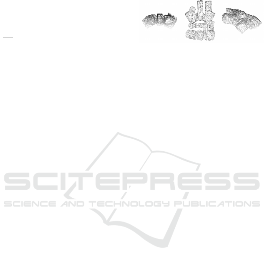
This mechanism is efﬁcient enough to generate

thousands of point clouds with primitive type labels

within hours. See Fig. 5 for an example.

5.1.2 Training

After data generation, our variant of PointNet++ is

trained on point clouds of about 100, 000 points each.

In addition to the point’s coordinates, we make use

of its estimated surface normal. To speed-up training,

Figure 5: A sample point cloud generated by our tool from

different views.

we extract points, which belong to the same primitive

from the initial point cloud in several subsets of 2048

points each. This procedure allows to handle larger

point cloud sizes while keeping inference and train-

ing times low. Additionally, we allow PointNet++ to

generalize further among the available points. Early

stopping prevents the model network from overﬁtting

to the training set. The prediction process is explained

in Section 4.2, primitive type detection.

5.2 Results of the Full Pipeline

We use 5 point clouds {PC1, . . . , PC5} with

{96.4k, 111.2k, 30.0k, 50.0k, 30.0k} points. The ﬁrst

three columns in Fig. 6 show the results of the inter-

mediate steps in the primitive type detection module,

whereas the last column shows the set of solid prim-

itives obtained at the end of the full pipeline. Please

note that the goal here is not to reconstruct a com-

plete solid model but instead to generate a set of sim-

ple solid primitives, describing the point cloud and

from which the model can be reconstructed, e.g. by

CSG operations. We measured wall-clock times for

the data sets shown in Fig. 6 on an Intel Core i7-

7600U @ 2.9GHz with 16GB RAM.

Results for the primitive type detection step are

shown in Fig. 7. Within this step, the per-point prim-

itive type prediction (Detection in Fig. 7) is the most

expensive in terms of computation times.

For the primitive ﬁtting step (see Fig. 8), the

RANSAC iterations (we used 3 iterations) are

the dominant factor contributing to the durations,

whereas the merge process is < 10ms for all data sets

and thus negligible. Please note that with clustering,

we are able to detect all relevant primitives for each

model.

The results of the solid primitive generation step

(wall-clock time and number of iterations) are de-

picted in Fig. 9. We used an unoptimized, single-

core implementation of the GA, which could eas-

ily be parallelized for better performance. We ran

the GA with a population size of 150 individuals,

a maximum cuboid set size of 75 (n

C max

), weights

(α = 1, β = 0.1, γ = 0.1) and a mutation and crossover

probability (p

, p

) of 0.4 for a maximum of 100 it-

GRAPP 2020 - 15th International Conference on Computer Graphics Theory and Applications

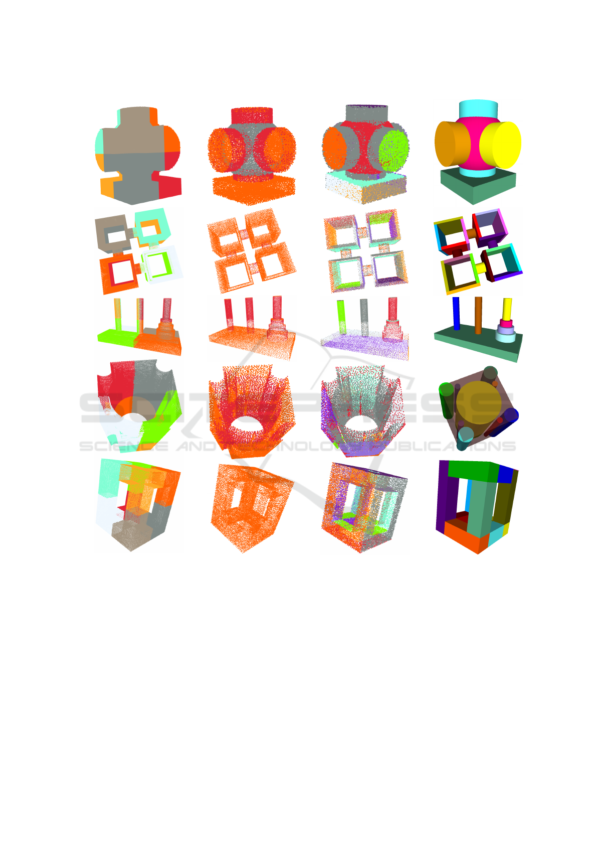
PC1PC2PC3PC4PC5

(a) Spatial Partitioning.

(b) Detection (red: cylinders,

grey: spheres, orange: planes).

(d) Final set of solid primitives.

Figure 6: Results of the different pipeline steps.

erations. Additionally, in case of 25 consecutive iter-

ations without score improvement, the GA terminates

as well. For data sets PC1 and PC2, the maximum

number of iterations has been reached (see Fig. 9).

However, in both cases, the GA converged to a result

containing all necessary cuboids, as can be observed

in Fig. 6d. Since the GA is a non-deterministic al-

gorithm, each run could result in potentially different

cuboid sets, all having the same ﬁtness function value.

Thus, for example, in the case of PC5, cuboids made

of different plane combinations could be obtained as

a possible result.

5.3 Comparison to Other Approaches

In Fig. 10 we compare the number of detected sur-

face primitives with and without clustering (as done

in primitive type detection). It shows that the primi-

tive ﬁtting step improves over plain RANSAC by in-

creasing robustness (the variance of the number of

A Hybrid Approach for Segmenting and Fitting Solid Primitives to 3D Point Clouds

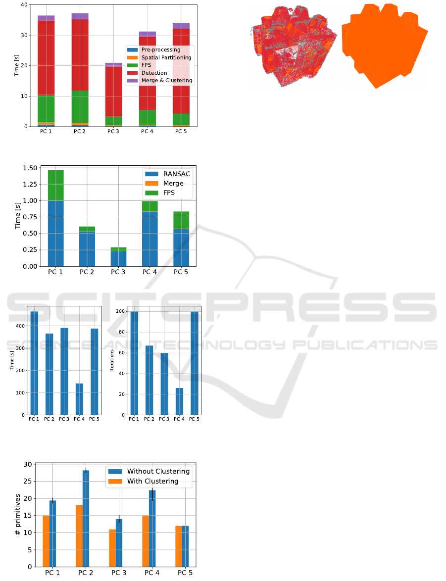
Figure 7: Timings for primitive type detection.

Figure 8: Timings for primitive ﬁtting.

Figure 9: Timings and number of iterations for solid primi-

tive generation.

Figure 10: Number of primitives with and without cluster-

ing. Variance is indicated by the black lines.

(a)

(b)

Figure 11: (a) Detection on a real-world scan severely cor-

rupted by noise. Some planar parts are erroneously assigned

to a different type. (b) Perfect planes detection on the man-

ually cleaned point cloud.

primitives over multiple runs is decreased) and de-

creasing the number of redundant, as well as poorly

ﬁtted primitives for all models with the exception of

PC5. For PC5, only planes need to be ﬁtted, which is

a comparatively simple task that does not beneﬁt from

additional clustering. Additionally, the solid primitive

generation step allows to generate solid primitives un-

like RANSAC.

Compared to existing deep learning-based tech-

niques, the proposed approach can handle larger point

clouds, does not rely on very speciﬁc training data

sets for particular model categories and does support

both, cuboids and capped quadric-based primitives

((Zou et al., 2017) and (Tulsiani et al., 2017) support

only cuboids, (Paschalidou et al., 2019) supports only

superquadrics and (Li et al., 2019) supports planes,

uncapped cylinders, uncapped cones and spheres).

5.4 Limitations

Here, we discuss issues found in the proposed ap-

proach that are left for future work.

Tolerance to Noise. The primitive type detection step

may fail on data corrupted by severe noise as shown in

Fig. 11a. For this example, a manual cleaning of the

data helps in detecting the correct types (Fig. 11b).

Please note that this manual pre-processing step was

not necessary for the evaluated data sets shown in

Fig. 6. We plan to improve our training data gener-

ator such that it implements a better scan simulation

instead of a simple mesh surface sampling with addi-

tional noise in order to increase robustness.

Redundant Primitives. Sometimes, our approach

can produce redundant cuboids, e.g. a cuboid that is

completely contained in another cuboid. This can be

controlled by tuning γ in (1).

Additionally, depending on the type of application

where the set of solid primitives produced by our ap-

proach is used, these problems may not be an issue at

all. One such example is when the set of solid primi-

tives is used as the input to a CSG tree reconstruction

GRAPP 2020 - 15th International Conference on Computer Graphics Theory and Applications

method such as (Fayolle and Pasko, 2016; Wu et al.,

2018; Du et al., 2018).

Missing Details. In some rare cases, ﬁne geometric

details are not reconstructed correctly with the pro-

posed approach. This can be mitigated by increasing

the point cloud density as well as the GA’s maximum

number of iterations. In addition, the objective func-

tion weights (Equation 1) can be tweaked for a spe-

ciﬁc data set. A reduction of parameter sensitivity is

planned for future work.

Unconnected Cylinders. Since the height of a cylin-

der is estimated using the associated point cloud, it

can happen that the cylinder is not connected to other

parts and small gaps appear between primitives. This

can be mitigated by adding cylinders to the GA to ﬁnd

their optimal capping planes.

6 CONCLUSION

In this paper, a hybrid primitive segmentation and ﬁt-

ting pipeline is proposed. Our approach is capable of

handling large point clouds in reasonable time. As fu-

ture work, we plan to tackle the limitations discussed

in Section 5.4. In addition, we plan to add extra shape

types, such as arbitrary convex polytopes.

REFERENCES

Attene, M., Falcidieno, B., and Spagnuolo, M. (2006). Hi-

erarchical mesh segmentation based on ﬁtting primi-

tives. The Visual Computer, 22(3):181–193.

Benk

o, P., Martin, R. R., and V

arady, T. (2001). Algorithms

for reverse engineering boundary representation mod-

els. Computer-Aided Design, 33(11):839–851.

Breunig, M. M., Kriegel, H.-P., Ng, R. T., and Sander, J.

(2000). Lof: Identifying density-based local outliers.

SIGMOD Rec., 29(2):93–104.

Cohen-Steiner, D., Alliez, P., and Desbrun, M. (2004). Vari-

ational shape approximation. ACM Trans. Graphics,

3(23):905–914.

Czerniawski, T., Sankaran, B., Nahangi, M., Haas, C., and

Leite, F. (2018). 6D DBSCAN-based segmentation of

building point clouds for planar object classiﬁcation.

Automation in Construction, 88(December 2017):44–

58.

Du, T., Inala, J. P., Pu, Y., Spielberg, A., Schulz, A., Rus,

D., Solar-Lezama, A., and Matusik, W. (2018). In-

versecsg: Automatic conversion of 3d models to csg

trees. ACM Trans. Graph., 37(6):213:1–213:16.

Ester, M., Kriegel, H.-P., Sander, J., and Xu, X. (1996).

A density-based algorithm for discovering clusters a

density-based algorithm for discovering clusters in

large spatial databases with noise. In Proceedings of

the Second International Conference on Knowledge

Discovery and Data Mining, KDD’96, pages 226–

231. AAAI Press.

Fayolle, P.-A. and Pasko, A. (2016). An evolutionary ap-

proach to the extraction of object construction trees

from 3d point clouds. Computer-Aided Design, 74:1–

17.

Fischler, M. A. and Bolles, R. C. (1981). Random sample

consensus: a paradigm for model ﬁtting with appli-

cations to image analysis and automated cartography.

Communications of the ACM, 24(6):381–395.

Friedrich, M., Cuevas, F. G., Sedlmeier, A., and Ebert, A.

(2019). Evolutionary generation of primitive-based

mesh abstractions. In Proceedings of WSCG 2019.

Fukuda, K. and Prodon, A. (1995). Double description

method revisited. In Combinatorics and Computer

Science.

Genova, K., Cole, F., Vlasic, D., Sarna, A., Freeman, W. T.,

and Funkhouser, T. (2019). Learning shape templates

with structured implicit functions. arXiv preprint

arXiv:1904.06447.

Kaiser, A., Zepeda, J. A. Y., and Boubekeur, T. (2019). A

survey of simple geometric primitives detection meth-

ods for captured 3d data. Computer Graphics Forum,

38(1):167–196.

Kalogerakis, E., Hertzmann, A., and Singh, K. (2010).

Learning 3d mesh segmentation and labeling. ACM

Trans. Graph., 29(4):102:1–102:12.

Kim, V. G., Li, W., Mitra, N. J., Chaudhuri, S., DiVerdi,

S., and Funkhouser, T. (2013). Learning part-based

templates from large collections of 3d shapes. ACM

Trans. Graph., 32(4):70:1–70:12.

Lavou

e, G., Dupont, F., and Baskurt, A. (2005). A new

CAD mesh segmentation method, based on curvature

tensor analysis. Computer-Aided Design, 37(10):975–

987.

Le, T. and Duan, Y. (2017). A primitive-based 3d segmenta-

tion algorithm for mechanical cad models. Computer

Aided Geometric Design, 52:231–246.

Li, L., Sung, M., Dubrovina, A., Yi, L., and Guibas, L. J.

(2019). Supervised ﬁtting of geometric primitives to

3d point clouds. In Proceedings of the IEEE Con-

ference on Computer Vision and Pattern Recognition,

pages 2652–2660.

Li, M., Wonka, P., and Nan, L. (2016). Manhattan-world

urban reconstruction from point clouds. In ECCV.

Li, Y., Wu, X., Chrysathou, Y., Sharf, A., Cohen-Or, D.,

and Mitra, N. J. (2011). Globﬁt: Consistently ﬁtting

primitives by discovering global relations. ACM trans-

actions on graphics (TOG), 30(4):52.

Marshall, D., Lukacs, G., and Martin, R. (2001). Ro-

bust segmentation of primitives from range data in

the presence of geometric degeneracy. IEEE Trans-

actions on Pattern Analysis and Machine Intelligence,

23(3):304–314.

Monszpart, A., Mellado, N., Brostow, G. J., and Mitra, N. J.

(2015). RAPter: Rebuilding man-made scenes with

regular arrangements of planes. ACM Trans. Graph.,

34(4):103:1–103:12.

Nan, L. and Wonka, P. (2017). Polyﬁt: Polygonal surface

reconstruction from point clouds. In Proceedings of

A Hybrid Approach for Segmenting and Fitting Solid Primitives to 3D Point Clouds

the IEEE International Conference on Computer Vi-

sion, pages 2353–2361.

Oesau, S., Lafarge, F., and Alliez, P. (2016). Planar shape

detection and regularization in tandem. Computer

Graphics Forum, 35(1):203–215.

Paschalidou, D., Ulusoy, A. O., and Geiger, A. (2019). Su-

perquadrics revisited: Learning 3d shape parsing be-

yond cuboids. In Proceedings of the IEEE Conference

on Computer Vision and Pattern Recognition, pages

10344–10353.

Qi, C. R., Su, H., Mo, K., and Guibas, L. J. (2017a). Point-

net: Deep learning on point sets for 3d classiﬁcation

and segmentation. In Proceedings of the IEEE Con-

ference on Computer Vision and Pattern Recognition,

pages 652–660.

Qi, C. R., Yi, L., Su, H., and Guibas, L. J. (2017b). Point-

net++: Deep hierarchical feature learning on point sets

in a metric space. In Advances in neural information

processing systems, pages 5099–5108.

Schnabel, R., Wahl, R., and Klein, R. (2007). Efﬁcient

ransac for point-cloud shape detection. Computer

graphics forum, 26(2):214–226.

Shamir, A. (2008). A survey on Mesh Segmentation Tech-

niques. Computer Graphics Forum, 27(6):1539–1556.

Shamos, M. I. (1978). Computational Geometry. PhD the-

sis, Yale, New Haven, CT, USA. AAI7819047.

Tulsiani, S., Su, H., Guibas, L. J., Efros, A. A., and Malik,

J. (2017). Learning shape abstractions by assembling

volumetric primitives. In Proceedings of the IEEE

Conference on Computer Vision and Pattern Recog-

nition, pages 2635–2643.

Vanco, M. and Brunnett, G. (2004). Direct segmentation of

algebraic models for reverse engineering. Computing,

72(1):207–220.

arady, T., Benko, P., and Kos, G. (1998). Reverse en-

gineering regular objects: simple segmentation and

surface ﬁtting procedures. Int. J. of Shape Modeling,

3(4):127–141.

Wu, Q., Xu, K., and Wang, J. (2018). Constructing 3d csg

models from 3d raw point clouds. Computer Graphics

Forum, 37(5):221–232.

Xiao, J. and Furukawa, Y. (2014). Reconstructing the

world’s museums. International Journal of Computer

Vision, 110(3):243–258.

Zhirong Wu, Song, S., Khosla, A., Fisher Yu, Lin-

guang Zhang, Xiaoou Tang, and Xiao, J. (2015).

3d shapenets: A deep representation for volumetric

shapes. In 2015 IEEE Conference on Computer Vision

and Pattern Recognition (CVPR), pages 1912–1920.

Zou, C., Yumer, E., Yang, J., Ceylan, D., and Hoiem, D.

(2017). 3d-prnn: Generating shape primitives with

recurrent neural networks. In Proceedings of the IEEE

International Conference on Computer Vision, pages

900–909.

GRAPP 2020 - 15th International Conference on Computer Graphics Theory and Applications