
Analysing Usage of Harvested Energy in Wireless Sensor Networks:
A Geo/Geo/1/K Approach
O. P. Angwech
1 a
, A. S. Alfa
2,3 b
and B. T. J. Maharaj
1 c
1
Department of Electrical, Electronic and Computer Engineering, University of Pretoria, Pretoria 0002, South Africa
2
Department of Electrical and Computer Engineering, University of Manitoba, Winnipeg, Manitoba, Canada
3
Department of Electrical, Electronic and Computer Engineering, (CSIR/UP SARChI ASN Chair), University of Pretoria,
Pretoria 0002, South Africa
Keywords:
Wirless Sensor Networks, Energy Harvesting, Markov Chain.
Abstract:
A model that considers energy storage and usage in data transmission in Wireless Sensor Network applications
is proposed. The system is modelled as a Geo/Geo/1/k system and analysed using standard finite Markov chain
model tools. The stationary distribution of the queue length is obtained. In the model, the harvested energy
is stored in a buffer and used as required by the packets. In addition to energy usage by the packets, leakage
of energy is captured at each state. A situation that involves high and low priority data transmission is also
captured in the model. For evaluation, the effects of the system parameters on the performance measures are
analysed. The results show that the model accurately captures the energy usage and it can be used for the
management of harvested energy in Wireless Sensor Networks.
1 INTRODUCTION
The growth of Wireless Sensor Networks (WSNs) in
the last decade has been aided by their use in various
applications some of which are found in areas such as
security, military systems, healthcare, transportation
systems, agriculture and environment. WSNs consist
of several tiny sensor nodes that are densely deployed
either within an event or close to it. These sensor
nodes consist of communicating, data processing and
sensing components which maybe required to fit into
a match-box sized module (Akyildiz et al., 2002). In
addition to size, other constraints on sensor nodes in
WSNs include; low power consumption, size depend-
ing on the application, able to adapt to the environ-
ment, dispensable, have low production costs, operate
unattended and be autonomous as they are often inac-
cessible (Akyildiz et al., 2002). The size constraint
of sensor nodes makes power a scarce resource in the
nodes as they are usually powered by small lithium
cells batteries (usually 2.5cm in diameter and 1cm
thick) which have limited capacity (Akyildiz et al.,
2002; Vardhan et al., 2000). These batteries are usu-
a
https://orcid.org/0000-0002-5071-5181
b
https://orcid.org/0000-0002-6486-2908
c
https://orcid.org/0000-0002-3703-3637
ally affected by the energy usage pattern and active-
ness level of the sensor nodes and can sustain the net-
work for long or short periods.
In order to extend the network lifetime, energy
harvesting has been one of the exploited areas in
WSNs (Tadayon et al., 2013). Energy harvesting
models play a very important role in the design and
evaluation of energy harvesting systems. The mod-
els are primarily divided into three groups, namely,
deterministic, stochastic and other models (Ku et al.,
2016). Deterministic models are suitable for applica-
tions with predictable or slow varying energy sources
and depend on the accurate prediction of the energy
profile over a long period of time. However, mod-
elling mismatch is encountered as prediction inter-
vals are increased. In other models, RF signals that
are artificially generated by external devices are con-
sidered (Mouapi et al., 2017). The RF signals are
either random or deterministic. The amount of en-
ergy harvested is dependent on two factors, namely,
the transmitted power of transmitters and the chan-
nels from the transmitters to the harvesting receivers.
These factors introduce a trade-off between energy
and information transfer in wireless sensor networks.
In a stochastic model, the energy renewal process is
considered to be random. Non-causal energy state is
not needed, hence making it suitable for applications
Angwech, O., Alfa, A. and Maharaj, B.
Analysing Usage of Harvested Energy in Wireless Sensor Networks: A Geo/Geo/1/K Approach.
DOI: 10.5220/0008869500710077
In Proceedings of the 9th International Conference on Sensor Networks (SENSORNETS 2020), pages 71-77
ISBN: 978-989-758-403-9; ISSN: 2184-4380
Copyright
c
2022 by SCITEPRESS – Science and Technology Publications, Lda. All rights reserved
71

that have an unpredictable energy state. Some of the
stochastic models used in energy harvesting applica-
tions include Bernoulli models, the Poisson process
and the exponential process (Ku et al., 2016).
Many studies have been done in queueing theory
and energy harvesting. Some works have focused on
the self-sustainability of energy-harvesting networks
with infinite battery capacity, stochastic arrivals of en-
ergy and a fixed rate of energy consumption (Guru-
acharya and Hossain, 2018). Others have focused on
the design of the system in terms of the required sizes
of the data and energy buffers (Zhang et al., 2013).
In other studies, priority scheduling is employed
in the integration of different types of traffic in
packet-based networks and is classified in two ways,
pre-emptive and non-pre-emptive (Walraevens et al.,
2011). In a pre-emptive system, the service is in-
terrupted once a high priority event enters the sys-
tem. On the other hand, in a non-pre-emptive system,
service is completed and thereafter the high priority
event is given service. In some works, the low pri-
ority events were subjected to a finite buffer and the
high priority buffer was infinite (Jolai et al., 2010).
In others, a two dimensional Markov chain is used to
develop the state-transition matrix for the model (Ma
et al., 2013).
Although research has been done on stochastic
models, specifically, queueing models for energy har-
vesting in WSNs, some of these models do not ac-
curately capture the energy drawing process (Zhang
and Lau, 2015; Jeon and Ephremides, 2015; Ashraf
et al., 2017; Dudin and Lee, 2016; Ku et al., 2015).
The energy needs of nodes met by a combination of
energy harvesting and a connection to the mains as
a back-up when the batteries have been depleted has
been studied (Gelenbe, 2015). This work assumes
that the arrival of data packets and energy tokens fol-
low a Poisson process and the rate at which energy is
harvested is slow in comparison to the rate at which
data is transmitted. In another study, a sensor node ca-
pable of energy harvesting was analysed and assumes
uncertainty in energy harvesting, depletion and data
acquisition. The sensor node was modelled as a two
dimensional Markov chain with one queue for the en-
ergy and the other for the data. This study assumes
that arrival rates of energy and data follow a Poisson
process (De Cuypere et al., 2018).
In another study, the effect of energy loss through
battery or capacitor leakage and standby operation is
studied. The arrival rates of energy and data packets
are assumed to follow a Poisson process and the leak-
age is represented as an exponential decay (Gelenbe
and Kadioglu, 2015).
In this paper, the major contributions are as fol-
lows. Three models are proposed, two of which have
two queues, the data queue and the energy queue. The
third model is the priority model and has two data
buffers, high priority (HP) and low priority (LP) data
packets. The energy units are modelled as tokens re-
quired by packets in order to get processed. The ar-
rival of both data packets and energy tokens are con-
sidered to be random. Both the data packets and en-
ergy tokens are considered to be discrete. One energy
token is a discrete unit and is the minimum amount
of energy required to transmit one data packet. The
proposed model is a three-dimensional Markov chain
with leakage is imposed on the energy queue. To the
author’s knowledge, a leakage of tokens at different
transitions has not been implemented. This work aims
to capture the accumulation, the leakage and the dis-
sipation of energy in the model.
2 SYSTEM MODEL
The sever is modelled as a single node queue in dis-
crete time and the following assumptions are made,
the data and energy buffers are finite i.e. the number
of tokens and packets that can be queued is limited.
One bit of data is referred to as a packet and one unit
of energy is referred to as a token.
Figure 1: System Model.
For the token analysis, the following assumptions
are made, each token gives permission for the trans-
mission of one packet. If a token is waiting in the
energy buffer, an arriving packet removes it from the
buffer and enters the network. If there are no to-
kens waiting in the energy buffer, the incoming packet
waits in the data buffer of a given size, when the buffer
is at its maximum capacity the packet is lost. Simi-
larly if the energy buffer is full, the tokens are lost.
SENSORNETS 2020 - 9th International Conference on Sensor Networks
72

3 QUEUEING ANALYSIS
3.1 Model
3.1.1 Description
The model suggests that the discrete inter-arrival
times of the packets and tokens follow a geometric
distribution with probabilities a, arrival of a packet
and b, arrival of a token. Let ¯a = 1 − a,
¯
b = 1 − b,
C
T
be the transpose of matrix C and B
T
01
be the trans-
pose of matrix B
01
. The system is considered to be
first-come-first-serve (FCFS) unless stated otherwise.
Figure 1 shows the proposed model.
3.1.2 State Space
The state space of the system in Figure 1 is described
by a two-dimensional Markov chain, (I
n
, J
n
), n ≥ 0.
I
n
is the number of packets in the buffer at time n,
0 ≤ I
n
≤ F, J
n
is the number of tokens in the buffer at
time n, 0 ≤ J
n
≤ K , K represents the token buffer and
F represents the packet buffer.
3.1.3 Transition Matrix
The transition matrix, P, is a classical Quasi-Birth-
Death (QBD) matrix. An entry in the matrix repre-
sents the transition from one sate given in the row to
the next state given in the corresponding column. An
absence of an entry in the matrix implies that the two
states are not accessible to each other. By applying
the lexicographical order for the state space, the prob-
ability transition matrix P is obtained as follows.
P =
B C
E A
1
A
0
A
2
A
1
A
0
.
.
.
.
.
.
.
.
.
A
2
A
1
+ A
0
, (1)
where
B =
ab + ¯a
¯
b ¯ab
a
¯
b ab + ¯a
¯
b ¯ab
.
.
.
.
.
.
.
.
.
a
¯
b ab + ¯a
,
C =
a
¯
b 0 ··· 0
T
,
E =
¯ab 0 · · · 0
,
A
1
= ab + ¯a
¯
b, A
0
= a
¯
b, A
2
= ¯ab.
For the stable system x is obtained such that
x = xP, x1 = 1, (2)
where
x = [x
00
, x
01
, x
02
, ..x
0K
, x
10
, x
20
, x
30
, ..x
N0
].
In the analysis of the performance of a queueing sys-
tem, key system characteristics are specified namely,
the arrival and service times (Alfa, 2010). The perfor-
mance measures are obtained using Equation 3. The
mean number of packets and tokens in the system are
given as follows respectively.
E
p
[x] =
N
∑
i=1
ix
i,0
, E
t
[x] =
K
∑
j=0
jx
0, j
.
(3)
3.2 Model Including Leakage
To cater for energy leakage in the system, a parame-
ter θ is introduced in the system. Energy leakage is
expected when there is at least one token in the sys-
tem. An assumption is made, when a token arrives, it
stays until the next transition (at least one unit) before
it leaks. The probability of leakage is θ and that of no
leakage is 1 − θ. K is the token buffer. The probabil-
ity of having k tokens leak when there are n tokens at
time n in the system is a binomial distribution given
as follows.
l
n,k
=
n
k
θ
k
(1 − θ)
n−k
, n ≥ k. (4)
The state space of this model is described in section
3.1.2.
3.2.1 Transition matrix
The probability transition matrix, P, for this model is
obtained using equation 1.
where
B =
B
00
00
B
00
01
B
01
00
B
01
01
B
01
02
.
.
.
.
.
.
.
.
.
.
.
.
B
0K
00
B
0K
01
B
0K
02
· · · B
0K
0K
,
with
B
0n
00
= (ab + ¯a
¯
b)l
n,n
+ a
¯
bl
n,n−1
B
0n
01
= ¯abl
n,n
+ (ab + ¯a
¯
b)l
n,n−1
+ a
¯
bl
n,n−2
B
0n
02
= ¯abl
n,n−1
+ (ab + ¯a
¯
b)l
n,n−2
+ a
¯
bl
n,n−3
B
0K
0K
= a
¯
bl
K,1
+ (ab + ¯a
¯
b)l
K,K−K
+ a
¯
bl
K,K−K
where
C =
B
00
10
B
01
10
· · · B
0K
10
T
,
with
B
0n
10
= a
¯
bl
n,n
, E =
¯ab 0 · · · 0
,
A
1
= ab + ¯a
¯
b, A
0
= a
¯
b, A
2
= ¯ab.
The performance measures are obtained using equa-
tions 2 and 3.
Analysing Usage of Harvested Energy in Wireless Sensor Networks: A Geo/Geo/1/K Approach
73

3.3 Priority Model
3.3.1 Description
A system with two classes of packets arriving accord-
ing to the Bernoulli process is considered with prob-
abilities a
H
, arrival rate of High priority (HP) and a
L
,
arrival rate of Low priority (LP) packets. Figure 1 is
modified to cater for the priority. The priority model
has two separate packet buffers, one for the HP pack-
ets and the other for LP packets and is modelled as
a Geo/Geo/1 pre-emptive system which considers the
pre-emptive resume discipline.
The service discipline is as follows. No LP pri-
ority can start receiving service unless there is no
HP packet in the system and, if a LP packet is re-
ceiving service (in the absence of a HP packet in the
system), the service of this LP packet will be inter-
rupted at the arrival of a HP packet occurring before
the completion of the LP service. There is a possi-
bility of having up to two packets of each type arriv-
ing since we are dealing with discrete time. Hence,
the probability of arrivals of i type HP and j type
LP is defined as a
i
,
j
, i = 0, 1; j = 0, 1. For exam-
ple, a
0,0
= (1 − a
H
)(1−a
L
), a
0,1
= (1 − a
H
)a
L
, a
1,0
=
a
H
(1 − a
L
), a
1,1
= a
H
a
L
.
3.3.2 State Space
The state space of the model is described by a three-
dimensional Markov chain, (I
n
, J
n
, K
n
), n ≥ 0, I
n
is the
number of HP packets in the buffer at time n, 0 ≤ I
n
≤
M, J
n
is the number of LP packets in the buffer at time
n, 0 ≤ J
n
≤ N, K
n
is the number of tokens in the buffer
at time n, 0 ≤ K
n
≤ K. K represents the token buffer,
M represents the HP packet buffer and N represents
the finite LP buffer. To cater for leakage of tokens in
the system, equation 5 is used.
3.3.3 Transition Matrix
The transition matrix, P
l
, is given as follows.
P
l
=
B C
E A
1
A
0
A
2
A
1
A
0
A
2
A
1
A
0
.
.
.
.
.
.
.
.
.
A
2
A
1
+ A
0
, (5)
where
B =
B
00
B
01
B
2
B
1
B
0
B
2
B
1
B
0
.
.
.
.
.
.
.
.
.
B
2
B
1
+ B
0
,
with
B
00
=
B
000
000
B
000
001
B
001
000
B
001
001
B
001
002
B
002
000
B
002
001
B
002
002
B
002
003
.
.
.
.
.
.
.
.
.
.
.
.
B
00K
000
B
00K
001
B
00K
002
B
00K
003
· · · B
00K
00K
,
with
B
00n
000
= (a
1,0
b + a
0,1
b + a
0,0
¯
b)l
n,n
+ a
1,1
¯
bl
n,n−1
+
(a
1,0
¯
b + a
0,1
¯
b)l
n,n−2
+ a
1,1
¯
bl
n,n−2
B
00n
001
= a
0,0
bl
n,n
+ (a
1,0
b + a
0,1
b + a
0,0
¯
b)l
n,n−1
+
a
1,1
¯
bl
n,n−2
+ (a
1,0
¯
b + a
0,1
¯
b)l
n,n−3
+
a
1,1
¯
bl
n,n−3
B
00K
00(K−1)
= a
0,0
bl
K,K−(K−2)
+
(a
1,0
b + a
0,1
b + a
0,0
¯
b)l
K,K−(K−1)
+ a
1,1
bl
K,(K−K)
B
00K
00K
= a
0,0
bl
K,K−(K−1)
+ (a
1,0
b + a
0,1
b + a
0,0
¯
b)l
K,K−K
+ (a
1,0
¯
b + a
0,1
¯
b)l
K,K−K
B
2
= a
0,0
b, B
1
= a
0,1
b + a
0,0
¯
b, B
0
= a
0,1
¯
b,
B
01
=
B
000
010
B
001
010
B
002
010
· · · B
00K
010
T
,
with
B
00n
010
= (a
1,0
¯
b + a
1,1
b)l
n,n
C =
B
000
100
B
000
110
B
001
100
B
001
110
B
002
100
B
002
110
.
.
.
.
.
.
B
00K
100
B
00K
110
C
2
C
1
C
0
C
2
C
1
C
0
.
.
.
.
.
.
.
.
.
C
2
C
1
+C
0
,
with
B
00n
100
= (a
1,0
¯
b + a
1,1
¯
b)l
n,n
B
00n
110
= (a
1,0
¯
b + a
0,1
¯
b)l
n,n−1
+ a
1,1
¯
bl
n,n−1
SENSORNETS 2020 - 9th International Conference on Sensor Networks
74

C
2
= a
1,0
b, C
1
= a
1,0
¯
b + a
1,1
b, C
0
= a
1,1
¯
b,
E =
E
1
· · · 0 E
0
.
.
.
.
.
. E
1
E
0
.
.
.
.
.
. E
1
E
0
.
.
.
.
.
.
.
.
.
.
.
.
0 · · · 0 E
1
+ E
0
,
with
E
1
= a
0,0
b, E
0
= a
0,1
b,
A
1
=
A
1
1
A
0
1
A
1
1
A
0
1
A
1
1
A
0
1
.
.
.
.
.
.
A
1
1
+ A
0
1
,
with
A
1
1
= a
1,0
b + a
0,0
¯
b, A
0
1
= a
1,1
b + a
0,1
¯
b,
A
0
=
A
1
0
A
0
0
A
1
0
A
0
0
A
1
0
A
0
0
.
.
.
.
.
.
A
1
0
+ A
0
0
,
with
A
1
0
= a
1,0
¯
b, A
0
0
= a
1,1
¯
b,
A
2
=
A
1
2
A
0
2
A
1
2
A
0
2
A
1
2
A
0
2
.
.
.
.
.
.
A
1
2
+ A
0
2
,
with
A
1
2
= a
0,0
b, A
0
2
= a
0,1
b.
For a stable system we want to obtain x such that
equation 3 is satisfied.
where
x = [x
000
, x
001
, x
002
, ..x
00K
, x
010
, x
020
, x
030
, ..x
0N0
,
x
100
, x
200
, x
300
, ..x
M00
].
The performance measures are obtained using Equa-
tions 6 and 7. The mean number of tokens (E
t
[x]), LP
packets (E
l p
[x]) and HP packets (E
hp
[x]) in the system
are given as,
E
t
[x] =
K
∑
k=0
jx
0,0,k
(6)
E
l p
[x] =
N
∑
j=1
ix
0, j,0
E
hp
[x] =
M
∑
i=1
ix
i,0,0
(7)
4 RESULTS
Having developed the models and established the nu-
merical analysis, we now evaluate the performance of
a sensor node. We carry out simulations and obtain
results with the following parameters, a, the arrival
rate of packets, b, the arrival rate of tokens, F, the
packet buffer and K token buffer.
For the priority model the following parameters
are used, a
H
, the arrival rate of HP packets, a
L
, the
arrival rate of LP packets, M, HP packet buffer, N, LP
packet buffer and K token buffer.
4.1 Model
Figure 2 shows the mean number of tokens and pack-
ets in the system as the arrival rate of packets is var-
ied. The mean number of tokens decreases with an
increase in the mean number of packets in the system.
Figure 2: Effect of arrival rate of data packets on the mean
number of tokens and packets in the system. Here a is var-
ied, b = 0.6 , F = 200 and K = 100.
4.2 Model Including Leakage
Figure 3 shows the mean number of tokens and pack-
ets in the system as the rate of leakage is varied. The
mean number of tokens decreases with an increase in
the rate of leakage as packets are transmitted by the
available tokens and the unused ones leak.
4.3 Priority Model
Figure 4 shows the mean number of tokens and pack-
ets in the system as the arrival rate of the HP packets
is varied. The mean number of HP packets increases
with an increase in the arrival of HP packets, this is as
the rate of arrival of tokens is kept constant and will
get depleted after a specific period.
Analysing Usage of Harvested Energy in Wireless Sensor Networks: A Geo/Geo/1/K Approach
75
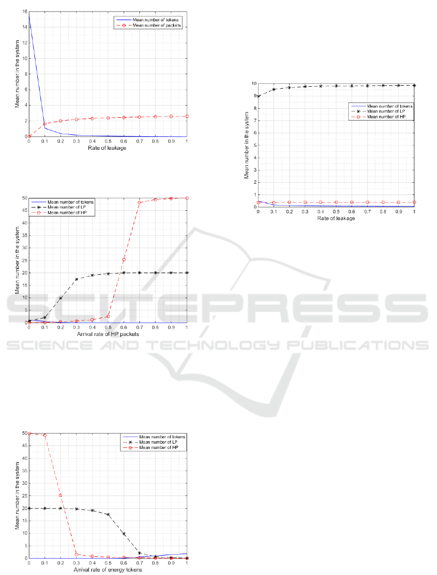
Figure 3: Effect of leakage on the mean number of tokens
and packets in the system. Here θ is varied, a = 0.52 b =
0.6, F = 72 and K = 18.
Figure 4: Effect of arrival rate of HP packets on the mean
number of tokens and packets in the system. Here a
H
is
varied, a
L
= 0.4, b = 0.6, θ = 0.4, M = 50, N = 20 and
K = 24.
Figure 5 shows the mean number of tokens and
packets in the system as the arrival rate of tokens in
the system is varied.
Figure 5: Effect of arrival rate of tokens on the mean num-
ber of tokens and packets in the system. Here b is varied,
a
H
= 0.2, a
L
= 0.4, θ = 0.4, M = 50, N = 20 and K = 24.
Figure 6 shows the mean number of tokens and
packets in the system the rate of the leakage in the
system is varied. The mean number of HP and LP
packets increases. The mean number of tokens de-
creases as there is leakage and usage by the packets
in the system.
Figure 6: Effect of leakage on the mean number of tokens
and packets in the system. Here θ is varied, a
H
= 0.2, a
L
=
0.4, b = 0.6, M = 50, N = 20 and K = 24.
5 DISCUSSION
An ideal system is modelled to have only packets and
tokens and the results are presented in Figure 2. It is
observed that both the token and packet buffers cannot
be full at the same time. When one buffer is full the
other is empty. In addition, as the arrival rate of data
packets increases the mean number of packets in the
system is observed to increase and the mean number
of tokens decreases. This is as each packet requires
a token to be processed, thereby decreasing the mean
number of tokens in the system as the arrival rate of
packets increases.
However, in a practical system, unused tokens of-
ten leak. This is captured in the model whose results
are presented in Figure 3. In this model, as the rate of
leakage increases the mean number of tokens in the
systems decreases. None of the buffers are full when
the rate of leakage is 0 as neither the arrival rate of
packets or tokens is 0 . When the probability of leak-
age is 0, this implies that the token buffer is full, how-
ever, this is not the case as there are packets (a = 0.52)
in the system that use some of the tokens. The token
buffer is therefore not full and the mean number of
tokens in the system is 97.4.
In addition to leakage, a practical system will have
emergency data (referred to as HP packets in this pa-
per) which has to be transmitted immediately. Leak-
age of energy and priority are captured in the model
whose results are presented in Figure 4, 5 and 6. As
SENSORNETS 2020 - 9th International Conference on Sensor Networks
76

the arrival rate of HP packets increases, the mean
number of tokens in the system decreases and the
mean number of HP and LP packets increases.
Finally we study the effect of leakage on the mean
number of tokens, HP and LP packets in the system
shown in Figure 6. As the rate of leakage increases,
the mean number of tokens in the system decreases
and the mean number of LP and HP packets increases.
The proposed models developed as Geo/Geo/1/k
systems shows that the proposed model illustrates the
effect of leakage on the mean number of tokens and
packets in the system.
6 CONCLUSIONS
In this paper, the performance of an energy harvest-
ing sensor node assuming data transmission and en-
ergy leakage was analysed. To this end, three models
were investigated. Two of the models had an energy
harvesting node which was modelled as a stochastic
system with two queues, one for data packets and the
other energy packets. We investigated the node when
a leakage is imposed on the energy buffer. To fur-
ther investigate the node, a third model was devel-
oped to observe the effect of priority. We showed
that the each of proposed systems can be described by
a Quasi-Birth-Death process (QBD). This allowed us
to obtain the performance measures using the matrix-
geometric methods. The simulations carried out re-
vealed the effect of leakage on the mean number of
tokens and packets in the system. Future work will
address the threshold case, when a threshold is im-
posed on the token buffer. When the token buffer is
below a specified level then the transmission of low
priority packets will be halted and only high priority
packets will be transmitted.
ACKNOWLEDGEMENTS
The authors would like to thank the South African Re-
search Chairs Initiative (SARChI) in Advanced Sen-
sor Networks (ASN) and SENTECH for their finan-
cial support in making this work possible.
REFERENCES
Akyildiz, I. F., Su, W., Sankarasubramaniam, Y., and Cayirci,
E. (2002). Wireless sensor networks: a survey. Computer
networks, 38(4):393–422.
Alfa, A. S. (2010). Queueing theory for telecommunications:
discrete time modelling of a single node system. Springer
Science & Business Media.
Ashraf, N., Asif, W., Qureshi, H. K., and Lestas, M. (2017).
Active energy management for harvesting enabled wire-
less sensor networks. In Wireless On-demand Network
Systems and Services (WONS), 2017 13th Annual Con-
ference on, pages 57–60. IEEE.
De Cuypere, E., De Turck, K., and Fiems, D. (2018). A queue-
ing model of an energy harvesting sensor node with data
buffering. Telecommunication Systems, 67(2):281–295.
Dudin, S. A. and Lee, M. H. (2016). Analysis of single-
server queue with phase-type service and energy harvest-
ing. Mathematical Problems in Engineering, 2016.
Gelenbe, E. (2015). Synchronising energy harvesting and data
packets in a wireless sensor. Energies, 8(1):356–369.
Gelenbe, E. and Kadioglu, Y. M. (2015). Energy loss through
standby and leakage in energy harvesting wireless sen-
sors. In 2015 IEEE 20th International Workshop on Com-
puter Aided Modelling and Design of Communication
Links and Networks (CAMAD), pages 231–236. IEEE.
Guruacharya, S. and Hossain, E. (2018). Self-sustainability of
energy harvesting systems: concept, analysis, and design.
IEEE Transactions on Green Communications and Net-
working, 2(1):175–192.
Jeon, J. and Ephremides, A. (2015). On the stability of ran-
dom multiple access with stochastic energy harvesting.
IEEE Journal on Selected Areas in Communications,
33(3):571–584.
Jolai, F., Asadzadeh, S., and Taghizadeh, M. (2010). A pre-
emptive discrete-time priority buffer system with par-
tial buffer sharing. Applied Mathematical Modelling,
34(8):2148–2165.
Ku, M.-L., Chen, Y., and Liu, K. R. (2015). Data-driven
stochastic models and policies for energy harvesting sen-
sor communications. IEEE Journal on Selected Areas in
Communications, 33(8):1505–1520.
Ku, M.-L., Li, W., Chen, Y., and Liu, K. R. (2016). Advances
in energy harvesting communications: Past, present, and
future challenges. IEEE Communications Surveys & Tu-
torials, 18(2):1384–1412.
Ma, Z., Guo, Y., Wang, P., and Hou, Y. (2013). The
Geo/Geo/1+1 queueing system with negative customers.
Mathematical Problems in Engineering, 2013.
Mouapi, A., Hakem, N., and Delisle, G. Y. (2017). A new ap-
proach to design of rf energy harvesting system to enslave
wireless sensor networks. ICT Express.
Tadayon, N., Khoshroo, S., Askari, E., Wang, H., and Michel,
H. (2013). Power management in smac-based energy-
harvesting wireless sensor networks using queuing anal-
ysis. Journal of Network and Computer Applications,
36(3):1008–1017.
Vardhan, S., Wilczynski, M., Portie, G., and Kaiser, W. J.
(2000). Wireless integrated network sensors (wins): dis-
tributed in situ sensing for mission and flight systems.
In Aerospace Conference Proceedings, 2000 IEEE, vol-
ume 7, pages 459–463. IEEE.
Walraevens, J., Fiems, D., and Bruneel, H. (2011). Perfor-
mance analysis of priority queueing systems in discrete
time. In Network performance engineering, pages 203–
232. Springer.
Zhang, F. and Lau, V. K. (2015). Delay-sensitive dynamic
resource control for energy harvesting wireless systems
with finite energy storage. IEEE Communications Maga-
zine, 53(8):106–113.
Zhang, S., Seyedi, A., and Sikdar, B. (2013). An analytical ap-
proach to the design of energy harvesting wireless sensor
nodes. IEEE Transactions on Wireless Communications,
12(8):4010–4024.
Analysing Usage of Harvested Energy in Wireless Sensor Networks: A Geo/Geo/1/K Approach
77
