
Sensor Fusion and Decision-making in the Cooperative
Search by Mobile Robots
Barouch Matzliach
1,3
, Irad Ben-Gal
1,3
and Evgeny Kagan
2,3
1
Dept. Industrial Engineering, Tel-Aviv University, Israel
2
Dept. Industrial Engineering, Ariel University, Israel
3
LAMBDA Laboratory, Tel-Aviv University, Israel
Keywords: Probabilistic Search, Bayesian Scheme, Multi-robot Systems, Sensor Fusion, Swarm Dynamics, Mobile
Robots.
Abstract: The paper addresses the problem of probabilistic search and detection of multiple targets by the group of
mobile robots that are equipped by a variety of sensors and are communicating with each other at different
levels. The goal is to define the trajectories of the robots in the group such that the targets are chased in
minimal time. The suggested solution model follows the occupancy grid approach, and sensor fusion is
implemented using a general Bayesian scheme with varying sensitivity of the sensors. The created control
algorithm was verified in three settings with different levels of communication and information sharing
between the robots and different levels of sensors' sensitivity. The suggested algorithms were implemented in
a software simulation to analyze and compare the different policies.
1 INTRODUCTION
The problem of search for a hidden object is one of
the oldest mathematical problems that attract both
theoretical and practical interest (Nahin, 2007). In its
basic formulation, this problem deals either with the
distribution of the search efforts or with the trajectory
of the searcher, such that provides a maximal
probability of detecting the target in a given time or
minimal time of certain detection of the target
(Stone,
1975).
Practical studies of the search problem were
initiated in 1942 as a result of the quest for the
detection of the submarines in Atlantic (Koopman,
1946). Then, the considerations were distributed to
the search of hidden moving targets (Washburn,
1983), and in most settings, there were suggested
optimal or near-optimal solutions of the problem; for
the overview, see, e.g. (Frost & Stone, 2001; Kagan
& Ben-Gal, 2013; Kagan & Ben-Gal, 2015;
Washburn, 1989).
However, with the development of mobile robots
and multi-robot systems, the problem of the search
was extended to the groups of autonomous agents
searching for single or multiple targets. In such a
setting, the activities of the agents strongly depend on
the communication between the agents and decisions
regarding the target made by each agent.
In the paper, we consider the problem of
probabilistic search and detection of multiple targets
by the group of mobile robots. Such a problem was
considered in (Pack, DeLima, Toussaint & York,
2009) in the framework of search by unmanned aerial
vehicles that required sophisticated navigation and
prediction techniques for control of the vehicles’
motion. In the earlier work (Vidal, Shakeria, Kim,
Shim & Sastry, 2002) in the field considered the
pursuit-evasion game of the team of the ground and
aerial vehicles that required to explore the terrain and
build its map.
We assume that the robots are equipped with
different sensors that can signal with both false
positive and false negative errors. The robots
communicate with each other and share information
regarding detected targets. In the paper, we consider
different levels of communications: from complete
sharing of the obtained date up to purely independent
activity without sharing information. The aim of the
research is to construct such control procedures that
provide detection of the targets in minimal time.
The suggested solution follows the simultaneous
location and mapping techniques (see, e.g. Siegwart
& Nourbakhsh, 2004), in particular – the occupancy
Matzliach, B., Ben-Gal, I. and Kagan, E.
Sensor Fusion and Decision-making in the Cooperative Search by Mobile Robots.
DOI: 10.5220/0008840001190126
In Proceedings of the 12th International Conference on Agents and Artificial Intelligence (ICAART 2020) - Volume 1, pages 119-126
ISBN: 978-989-758-395-7; ISSN: 2184-433X
Copyright
c
2022 by SCITEPRESS – Science and Technology Publications, Lda. All rights reserved
119
grid approach, where the map of the targets’
candidate points is created simultaneously with the
detection process and the robots’ motion (Elfes, 1987;
Elfes, 1990). The implemented sensor fusion follows
the general Bayesian scheme (Stone, Barlow &
Corwin, 1999). However, in order to bound the
influence of the false-positive detection errors, the
sensitivity of the sensors is specified dynamically
with respect to the status of the search.
The control algorithm implements three different
levels of communication and information sharing:
- each robot had complete information about the
data available to the other robots;
- the robots shared partial information;
- the robots acted independently without sharing
information.
As was expected, the independent actions of the
robots lead to the worst results in terms of the search
time and the best results are obtained in the case of
information sharing. In particular, while the robots
share complete information, then the search time
decreases exponentially with the increasing of the
sensors’ power down to a specific value and then
stays constant. In this case, we found the upper and
lower bounds for the probable sensor’s reliability
such that in these bounds, the search time is nearly
constant, and out of these bounds, the search time
increases exponentially.
The algorithms were implemented in the Python
programming language and the code can be directly
used for solving the real-world tasks of search and
detection by the groups of mobile robots.
2 THE CONSIDERED SCENARIO
OF COOPERATIVE SEARCH
Let us start with a general description of the
considered scenario of cooperative search.
Consider the number of mobile robots(agents)
searching for several stationary targets hidden in the
gridded domain. It is assumed that each searching
robot, as well as each target, can occupy only a single
cell of the grid. Each searching robot is equipped with
a variety of sensors that provide may be erroneous
information regarding the targets’ locations relative
to the robot’s location. The robots can communicate
and share information about the targets’ locations as
they have been perceived by the sensors. The goal is
to define the trajectories of the robots in the group and
their sensing activities such that all the targets will be
detected in minimal time.
In order to obtain the formal definition of the
presented scenario, including erroneous perception,
in addition to true targets that can be detected with a
certain probability, we introduce the dummy targets
that produce false alarms that can be perceived by the
robots’ sensors with certain probabilities.
It is clear that the presented scenario follows a
general framework of the probabilistic search (Stone,
1975; Stone, Barlow & Corwin, 1999); however, for
obtaining a practical solution, it requires several
heuristic approaches and reasonable assumptions. In
the next section, we start the consideration of
particular methods used in the suggested algorithm
and present the Bayesian sensor fusion that is used for
calculating the probabilities in the presence of false
alarms.
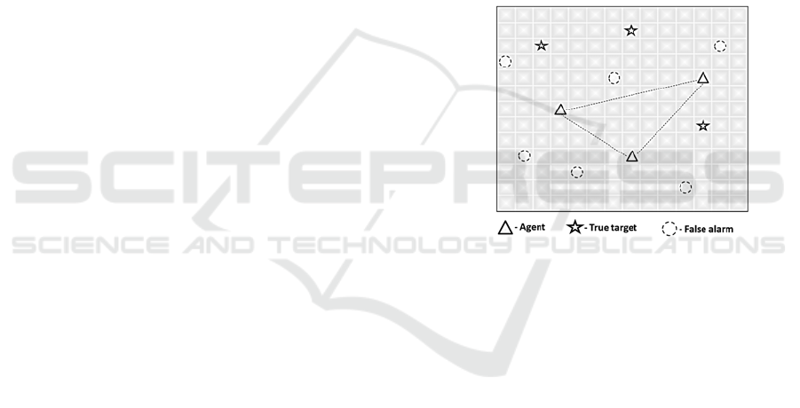
An example of the domain with true and dummy
targets is depicted in Figure 1.
Figure 1: An example of a search grid area with true and
dummy targets and several searching robots (agents).
3 UPDATING THE SENSOR
PROBABILITY MAP
Following the implemented approach of the
occupancy grid (Elfes, 1987; Elfes, 1990), the domain
perceived by the sensor is considered as a set of cells
, 1,2,…,∞. The state
of an ith cell is
defined as a discrete random variable with the values
1 that stands for the fact that the target is
located in the cell
or
0 that represents the
absence of the target in the cell
. It is clear that for
the probabilities of these two events in each cell
it
is assumed that
1
0
1
(1)
In other words, for each cell, it is associated with
a probability mass function that is estimated by the
sensors.
ICAART 2020 - 12th International Conference on Agents and Artificial Intelligence
120

As indicated above, following the assumption, the
domain includes true targets and dummy targets, and,
in each time, , they broadcast signals that represent
true and false alarms. The probabilities of perception
of these signals by the sensors are drawn with respect
to exponential distribution
|
⁄
(2)
where stands for the distance between the cell of
the target (true or dummy) and the cell, in which the
sensor is located, and is the sensor’s sensitivity.
Equation (2) forms a basis for the calculation of
the probability
,,
where
is a sensor of type installed on the th
agent
and scanning the cell
at time . This
calculation is as follows.
According to the Bayesian approach, the states
,
of the cells at time are estimated based on
information read by the sensor as follows. Denote by
̃
,the signal received by the sensor (more
precisely: by the sensor
of the agent
) at time
. Since in the considered scenario, the cell
at time
can be either occupied (
,
1) or not (
,
0), we say that ̃
,
1 if the sensor receives
information that
is occupied and ̃
,
0
otherwise. Then, the state probabilities of the cell
are:
,
1|
̃
,
1
,1
1
∙
̃
,
1│
,
1
∑
,1
∙
̃
,
1│
,
,
(3)
,
1|
̃
,
0
,1
1
∙
̃
,
0│
,
1
∑
,1
∙
̃
,
0│
,
.
(4)
These equations define the updating of the
probabilities map using new observations.
In addition, the signals received by the sensors can
be true or false alarms. Denote the positive alarm
received from the cell
by
1 and negative
alarm receives by the cell
by
0. Alarm
1 means, truly or not, that the cell
is
occupied, and alarm
0 means, truly or not,
that the cell
is empty.
Using the probability of receiving such alarms
defined equation (2), from the equations (3) and (4)
we obtain:
,
1|
̃
,
1
,1
1
∙
,
1│
,
1∙
∑
,1
∙
,
1│
,
∙
,
,
(5)
,
1|
̃
,
0
,1
1
∙1
,
1│
,
1∙
∑
,1
∙1
,
1│
,
∙
,
.
(6)
These equations allow calculating the occupation
probabilities at each time , given the probabilities at
the previous time 1 and the information obtained
by the sensors at time . At the initial time 1, the
probabilities are defined based on topographic data
and prior information or, in the worst case, can be
specified by a uniform distribution of the occupancy
grid.
4 SENSORS FUSION
As indicated above, it is assumed that each mobile
agent
is equipped with several sensors
of
different types of , and each sensor obtains
information from the cell
independently. Then,
sensors fusion allows filtering the events resulting in
false alarms and increasing the quality of detecting
real targets.
In the framework of the occupancy grid, sensor
fusion is conducted as follows. Consider two sensors
and
of the type
and
, respectively, installed at the same agent
. The
signals received by these sensors denote by ̃
,
and ̃
,
. Using these signals, the probability that
the state
,
of the cell
at time is
,
1
is defined as follows:
,
1|
̃
,
1,
̃
,
1
̃
,
│
,
∙
,
|
̃
,
∑
̃
,
│
,
∙
,
|
̃
,
,
.
(7)
If the agent
is equipped with independent
sensors
,
, …,
that perceive completely different types of signals, for
example, light, sound, ultrasound, and so far, then the
probability that the agent
on which these sensors
are installed detects the target in the cell
is
,
∏
∏
∏
,
(8)
where
,,
,
1
is the
probability defined by equations (5) and (6).
Sensor Fusion and Decision-making in the Cooperative Search by Mobile Robots
121
The presented equation is based on the approach
known as “independent opinion pool” under the
assumption that the sensors are independent and that
their reliabilities and accuracies are equivalent.
By the same manner can be fused the sensors
installed on different agents that result in global
probability.
∏
,
∏
,
∏
,
.
(9)
As a result, over the cells
, 1,2,…,, the
probabilities
,,
form the sensor
probabilities map for each sensor
of the agent
. The map is obtained by real-time updating of the
sensor's probabilities. The probabilities
,
form the agent
probabilities map, and the
probabilities
form the global probability
map.
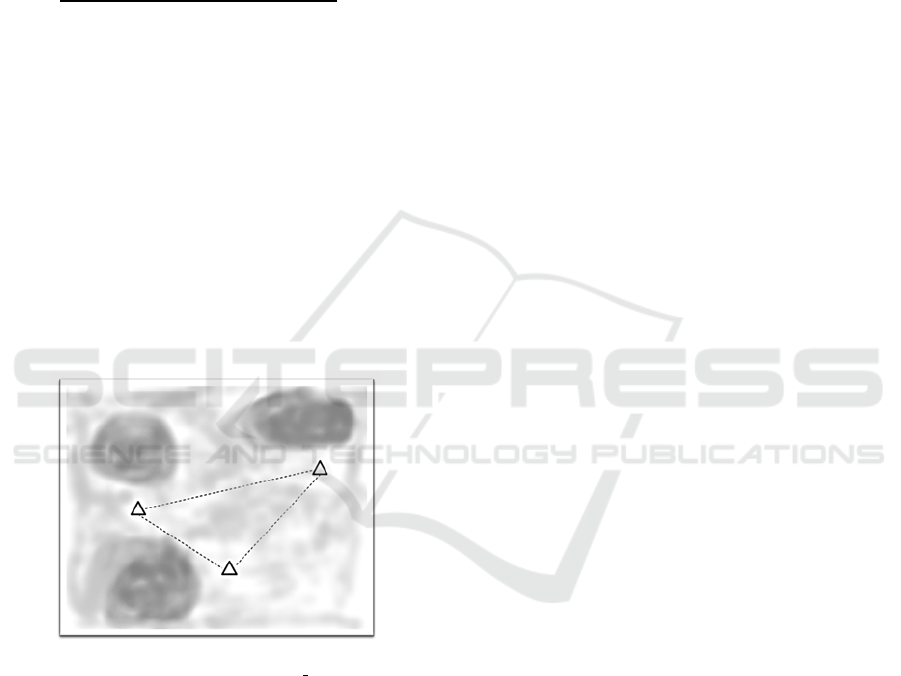
An example of a global probabilities map is
depicted in Figure 2. Dark color represents a higher
probability for target location.
Figure 2: Global probabilities map example.
5 PROBLEM FORMULATION
Now we are ready to formulate the considered
problem of search in the exact terms. As indicated in
the introduction, the goal is to define the trajectories
of the agents such that they detect the targets in
minimal time.
In general, such a problem can be considered from
two different directions:
1. The agents have to detect the targets and to reach
them. The search is terminated when all the targets
have been reached. In other words, the problem is
considered as the path-planning problem widely
accepted in the considerations of a search for
moving targets (Kagan & Ben-Gal, 2015).
2. The agents have to allocate the targets without
reaching them. The search process is terminated
when the positions of all the targets were achieved.
Such formulation follows classical considerations
of the search and screening problem that result in
the distribution of search efforts over the domain
(Stone, 1975).
Below, we focus on the first formulation. In this
scenario, the step of the search process is outlined as
follows.
1. At time , the agent
is located in the cell
and percepts the signals (that receives true and
false alarms) from the cells, in which the targets
can be located. The quality of sense depends on the
sensitivities of the agent’s sensors
and
the distances
,
between the agent’s cell
and the cells
, from which the alarms are
sent.
2. After receiving the signals, the sensor probability
maps
,,
, 1,2,…,, are updated.
3. The resulting sensor probability maps are
combined into the agent’s probability map
,
, 1,2,…,.
4. Following the considered control algorithms, there
are three possible scenarios:
4.1. If the agents act independently without
communication, the further decision about the next
step is obtained, based on the agent’s probability
map
,
, 1,2,…,.
4.2. If the agents can communicate, they can
share their maps with the other agents. In the case
of complete information sharing, each agent
creates a global probability map
,
1,2,…,, and makes a decision basing on this
map.
4.3. Otherwise, following partial maps obtained
from the other agents, the agent creates a local
probability map and makes a decision using this
map.
Thus, the problem consists of two questions:
1. What kind of communication (complete
information sharing, partial information sharing, or
independent activity) is better?
2. Given the probability map (global, partial or
individual), how the agent should choose its next
location?
In addition, we can allow the updating of the sensors'
sensitivity that allows decreasing the influence of
false alarms.
ICAART 2020 - 12th International Conference on Agents and Artificial Intelligence
122

6 SEARCH POLICIES
Let us start with the scenario in which the agents can
share complete information. In this case, at each time
each agent
is aware of its location
and the
probability map
,
, and about the global
probability map
, 1,2,…,.
Since for each cell in the grid (except boundary
cells) the agent has 9 possibilities: to stay in the
current cell or make a step to one of 8 neighboring
cells, the agent’s goal is to choose a possibility such
that it results in reaching the targets in minimum time.
The most information about the targets’ locations
is provided by the global probability map, and the
agent decides to move toward the highest probability
, 1,2,…,. In addition, since the
movements’ time is equivalent to the distance that the
agent moved, the agents’ choice should minimize this
distance. The simplest implementation of these two
assumptions is:
1
argmax
,…,
,
,
(10)
where
,
is the distance between the current
cell
occupied by the agent and the cell
.
The usage of a global probability map with
reasonable search policy, for example – with the
policy defined by equation (10), provides the best
results in terms of minimal search time than the usage
of partial or individual probability maps. However,
the usage of a global probability map requires either
transfer of all available information to a central
station and then broadcasting it to the agents or
transfer of all information to each agent and
processing it by the on-board computer. Obviously,
both options are rather problematic.
In order to decrease the quantity of transferred
information and of the computations, instead of a
global probability map, the partial or individual maps
can be used. In the first scenario, we assume that the
agent shares only those positions of the cells in which
the probabilities of detecting the targets are relatively
high. Such a technique allows decreasing uncertainty
in target locations and excluding some of the false
alarms. Formally, such sharing is implemented as
follows. The data are transferred among the sensors
of the same type installed on different agents
, 1,2,..,, and for this type the threshold
probability
∗
is specified. Over the agents we find
,
max
,…,
,,
,
(11)
and if
,
∗
, then the for each agent
the probability
,,
of the sensor of the
type is updated by:
,,
,
∙
,,
,
∙
,,
,
∙
,,
.
(12)
Such partial data sharing enhances the agent
probability map that allows better decisions even
using the simples rule defined by equation (10).
Finally, the same decision rule (10) was applied to
the individual agent’s probability map
,
,
1,2,…,. Such maps are created individually by
each agent and do not require communication
between the agents. Since such a scenario does not
imply information transfer and so is based on
decisions made using restricted data, it leads to the
longer search time.
7 SIMULATION RESULTS
The indicated three scenarios were studied by
numerical simulations. The methods and algorithms
were implemented using basic tools of the Python
programming language and the trials were run on
regular PC Intel I5 8265U.
In the simulations, the search is conducted over
the gridded domain of the size 8080 cells and both
searchers and the targets can occupy one cell. In the
illustrations below, we consider the group of 3 agents
searching for 3 targets. Each agent is equipped with
the sensors of 2 types. The starting positions of the
searchers are:
5,5
,
8,8
and
62,62
, and the
locations of the targets are:
65,76
,
75,70
and
75,78
.
In order to obtain the lower bound of search time,
we consider the scenario in which all the agents have
complete information about the targets’ locations and
move directly toward the targets. In this case, the
overall search time by three agents is
158.
Since this is the minimal possible time of the agents’
motion toward the targets, the other search scenarios
were compared with this time
.
In the first series of simulations, we considered
the search with constant sensors’ sensitivity
20 and different ratios of false alarms. The
implemented threshold probability is
∗
0.75 for
Sensor Fusion and Decision-making in the Cooperative Search by Mobile Robots
123
each type of the sensors. The results of the
simulations are summarized in Table 1.
Table 1: Search time in different scenarios with respect to
the frequency of false alarms.
False
alarms
per time
unit
Search time
Lower
bound
Global
map
Partial
data
sharing
Individual
maps
800 158 166 185 225
1600 158 188 202 321
3200 158 229 274 361
It is seen that, as it was expected, the best results
are provided using the global probability map. In this
case, the time of search is greater than its lower bound
only in 5% (for 800 false alarms per time unit), 19%
(for 1600 false alarms per time unit), and 45% (for
3200 false alarms).
The worthier results are obtained by the search with
partial information sharing. In this case, the time of
search is greater than its lower bound in 17% (for 800
false alarms per time unit), 28% (for 1600 false alarms
per time unit), and 73% (for 3200 false alarms).
Finally, the worst results were obtained in the
search with the use of individual probability maps
without information sharing. In this case, the time of
search is greater than its lower bound in 42% (for 800
false alarms per time unit), in 103% (for 1600 false
alarms per time unit), and in 128% (for 3200 false
alarms).
In all the scenarios, the increasing of search time
with the frequency of false alarms represents the
reaction of the agents to the greater uncertainty in the
data about the targets’ locations.
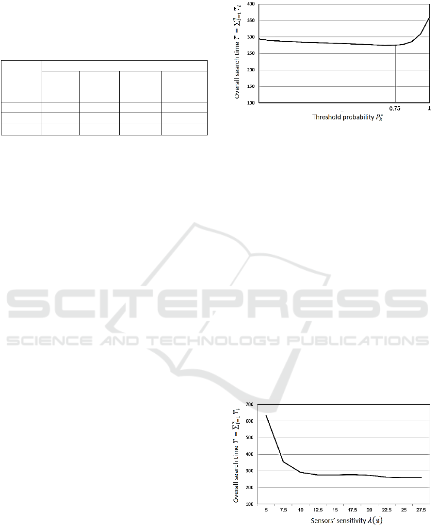
In the other series of simulations with the same
agents, we considered the dependence of search time
on the threshold probability
∗
in the scenarios with
partial information sharing between the agents. The
resulting dependence is shown in Figure 3.
In the figure, it is seen that the minimal time is
reached for the threshold's probability
∗
0.75 (it
was used in the above-described simulations). Notice
that for the values
∗
0.75, the search time
increases exponentially, while for the probabilities
∗
0.75 the time increasing is very slow and is
close to linear.
Thus, the value of optimal threshold probability
∗
is crucial for a search by the group of cooperating
agents and can completely change the search results.
However, in this paper, we do not address this
optimization problem and will define the probability
∗
heuristically based on the convexity of the
dependence of search time on this probability.
Figure 3: Dependence of the search time on the threshold
probability
∗
.
8 SENSORS WITH VARYING
SENSITIVITY
In the next simulations, we considered the dependence
of search time on the sensors’ sensitivity
on the
search time .
The greater sensitivity sensors enable to detect
more targets on greater distances from the agent.
However, more sensitive sensors are more expensive
and require more energy. In the case of active sensors,
the greater sensitivity also requires broadcasting
stronger signals that, especially for the military
robots, is not always possible.
Thus, in certain missions, the agents can be
equipped not with the best but with cheaper sufficient
sensors, that requires an exact definition of the
dependence of the search time on the sensitivity
. The resulting dependence obtained in numerical
simulations is shown in Figure 4.
Figure 4: Dependence of the search time on the sensors’
sensitivity
.
It is seen that the search time decreases
exponentially with the sensors’ sensitivity
such
that for the values
10 the greater sensitivity
has a minimal influence on the search time. That
ICAART 2020 - 12th International Conference on Agents and Artificial Intelligence
124

allows choosing the sensors with the sensitivity
~10 without loss of the search efficiency.
Finally, let us consider the real-time update of the
sensors’ sensitivity. Such updating enables tuning the
sensitivity with respect to the updates of the
probability map. Sensitivity updating is conducted as
follows.
Recall (see equation 11) that
,
stands
for maximum probability (over the agents) of
detecting the target at time by the sensor of type k.
Denote by
and by
, respectively, the upper and
the lower threshold probabilities. Then with respect
to these probabilities, the sensors’ sensitivity
at time 1 obtains the following value:
∙
,
,
,
,
⁄
,
,
(13)
where 1 is an updating coefficient.
The presented sensitivity updating allows
improvement of the search time. The results of
simulated search scenarios are summarized in Table 2.
Table 2: Search time in different scenarios with respect to
the sensors’ sensitivity.
Sensors’
sensitivity
Search time
Lower
bound
Global
map
Partial
data
sharing
Individual
maps
const
20
158 229 274 361
1.05 158 195 209 280
1.10 158 191 195 220
1.20 158 178 182 200
Here all the scenarios were simulated with 3200
false alarms are created per time unit; for the other false
alarm frequencies, the results follow the same tends.
The obtained results support the expectation that
greater sensitivity results in shorter search time and
demonstrate the effectiveness of dynamic sensitivity
tuning.
9 CONCLUSIONS
In the paper, we considered a probabilistic search for
multiple static targets by a group of agents acting in
the gridded domain. In opposite to most of the known
algorithms, we considered both false positive and false
negative detection errors.
For both types of errors, we considered three
levels of communication and information sharing:
- complete information sharing (the agents share
complete probability maps available to each of
them);
- partial information sharing (the agents share
the most robust parts of the available
probability maps);
- no information sharing (the agents act using
their own probability map).
In addition, in these scenarios, we assumed either
constant or varying sensors’ sensitivity that can be
changed online with respect to the target location
probabilities.
For the indicated scenarios, we developed new
models of decision making, sensor fusion and
information sharing. These models are simple enough
for practical implementation but, at the same time,
completely represent the data and control flows in the
system and include the processing of false positive
and false negative detection errors.
The developed models were implemented in the
Python software that was used in the simulations. The
simulations show that, as it was expected, the shortest
search times were demonstrated by the groups of
agents with complete information sharing and the
longest search times – by the groups without
information sharing. Partial information sharing
results in the intermediate time searches.
The online tuning of the sensors’ sensitivity
allows shorting the search times in all three
considered cases of information sharing; however, the
influence of the levels of information sharing still the
same.
The future research will address the problem of
building the probability maps, or, in other words, the
problem of detecting the targets without reaching
them in the grid. In this task, the movements of the
agents are governed by the expected information gain
for the targets’ locations and by their visibility, rather
than by detection probabilities. The results of this
research will complete the model and will allow using
the same terms at all the stages of the search process.
REFERENCES
Elfes, A., 1987, Sonar-based real-world mapping, and
navigation. IEEE J. Robotics and Automation, vol. 3,
no. 3, pp. 249-265.
Elfes, A., 1990, Occupancy grids: a stochastic spatial
representation for active robot perception. Proc. 6th
Conference on Uncertainty in Artificial Intelligence,
pp. 136-146.
Sensor Fusion and Decision-making in the Cooperative Search by Mobile Robots
125

Frost, J. R., Stone, L. D., 2001, Review of Search Theory:
Advances and Applications to Search and Rescue
Decision Support. Groton: US Coast Guard Research
and Development Centre.
Kagan, E., Ben-Gal, 2013, I. Probabilistic Search for
Tracking Targets. Chichester: Wiley & Sons, 2013.
Kagan, E., Ben-Gal, I., 2015, Search, and Foraging.
Individual Motion and Swarm Dynamics. Boca Raton:
Taylor & Francis.
Koopman, B. O., 1946, Search, and Screening. Operation
Evaluation Research Group Report, 56. Rosslyn,
Virginia: Centre for Naval Analysis.
Nahin, P. J., 2007, Chases and Escapes: The Mathematics
of Pursuit and Evasion. Princeton: Princeton University
Press.
Pack, D. J., De Lima, P., Toussaint, G. J., York, G., 2009,
Cooperative control of UAVs for localization of
intermittently emitting mobile targets. IEEE Trans.
Systems, Man, and Cybernetics, vol. 39, no. 4 pp. 959-
970.
Siegwart, R., 2004, Nourbakhsh, I. R. Introduction to
Autonomous Mobile Robots. Cambridge,
Massachusetts – London, England: The MIT Press.
Stone, L. D., 1975, Theory of Optimal Search. New York:
Academic Press.
Stone, L. D., Barlow, C. A., Corwin, T. L., 1999, Bayesian
Multiple Target Tracking. Boston: Artech House Inc.
Vidal, R., Shakeria, O., Kim, H., J., Shim, D., H., Sastry,
S., 2002, Probabilistic pursuit-evasion games: theory,
implementation and experimental evaluation. IEEE
Trans. Robotica and Automation, vol. 18, no. 5, pp.
662-669.
Washburn, A. R., 1983, Search for a moving target: the
FAB algorithm. Operations Research, vol. 31, no. 4, pp.
739-751.
Washburn, A. R., 1989, Search and Detection. Arlington,
VA: ORSA Books.
ICAART 2020 - 12th International Conference on Agents and Artificial Intelligence
126
