Comparison of the Optical Flow Quality for Video Denoising

Nelson Monz

1 a

and Javier S

anchez

2 b

CMLA,

Ecole Normale Sup

erieure, Universit

e Paris-Saclay, France

CTIM, Department of Computer Science, University of Las Palmas de Gran Canaria, Spain

Keywords:

Optical Flow, Video Denoising, Motion Trajectories, Temporal Filtering.

Abstract:

Video denoising techniques need to understand the motion present in the scenes. In the literature, many

strategies guide their temporal ﬁlters according to trajectories controlled by optical ﬂow. However, the quality

of these ﬂows is rarely investigated. In fact, there are very few studies that compare the behavior of denoising

proposals with different optical ﬂow algorithms. In that direction, we analyze several methods and their

performance using a general pipeline that reduces the noise through an average of the pixel’s trajectories. This

ensures that the denoising strongly depends on the optical ﬂow. We also analyze the behavior of the methods

at occlusions and illumination changes. The pipeline incorporates a process to get rid of these effects, so that

they do not affect the comparison metrics. We are led to propose a ranking of optical ﬂows methods depending

on their efﬁciency for video denoising, that mainly depends on their complexity.

1 INTRODUCTION

Video denoising (Boulanger et al., 2007; Arias and

Morel, 2018) is a key problem in image processing. It

generally requires a temporal noise ﬁltering guided by

motion trajectories. In this regard, optical ﬂow esti-

mation (Horn and Schunck, 1981; Lucas and Kanade,

1981) is quite useful because it provides consistent

information of the apparent displacement of the pix-

els through an image sequence. Therefore, the com-

puted solutions can be used to describe a trajectory

that guides the ﬁltering according to the vector ﬁelds

it provides.

Several works have been published to improve

the optical ﬂow computation in noisy images (Spies

and Scharr, 2001; Scharr and Spies, 2005), which is

one of the main challenges nowadays. Besides, the

current literature about video denoising assumes that

the motion estimation between frames is an advan-

tage (Liu and Freeman, 2010; Buades et al., 2016),

without exploring its inﬂuence in depth.

Nevertheless, in spite of research works like (Lars-

son and S

oderstr

om, 2015), there are not many arti-

cles that study the inﬂuence of the motion trajecto-

ries in video denoising. This is important as pointed

out in (Ehret et al., 2018), where the authors observe

the limitations of their results due to the optical ﬂow

https://orcid.org/0000-0003-0571-9068

https://orcid.org/0000-0001-8514-4350

method. In this sense, this work compares different

algorithms and analyze their inﬂuence when used for

video denoising. The purpose is not to improve the

current denoising methods but to observe the behav-

ior of accurate motion trajectories in the ﬁnal results.

We use a denoising frawework that averages the

pixel’s intensity through the trajectories obtained with

the corresponding optical ﬂow method. The rea-

son behind this strategy is to ensure that the accu-

racy of the denoising depends basically on the vec-

tor ﬁelds. We use a centered average to reduce the

impact of possible changes in the context of a scene.

In our experiments, we compare the optical ﬂow

methods proposed by Horn and Schunck (Horn and

Schunck, 1981), Brox et al. (Brox et al., 2004), Zach

et al. (Zach et al., 2007) and Monz

on et al. (Monz

et al., 2016). Arguably, an algorithm that uses tem-

poral information could be helpful to obtain consis-

tent trajectories. Thus, we also include in our exper-

iments the temporal method proposed in S

anchez et

al. (S

anchez et al., 2013) and a temporal extension of

the Brox et al. method.

2 DENOISING FRAMEWORK

Next, we brieﬂy describe the main features of the de-

noising framework used to compare the inﬂuence of

the optical ﬂow methods in noise reduction.

Monzón, N. and Sánchez, J.

Comparison of the Optical Flow Quality for Video Denoising.

DOI: 10.5220/0008767507170724

In Proceedings of the 15th International Joint Conference on Computer Vision, Imaging and Computer Graphics Theory and Applications (VISIGRAPP 2020), pages 717-724

ISBN: 978-989-758-402-2

717

In the ﬁrst step, we introduce additive white Gaus-

sian noise (AWGN), with standard deviation σ, to the

input sequence. Then, we compute the optical ﬂows

for the whole noisy sequence in both directions. For

each image i, the neighboring frames [i − n, i + n] are

warped to the central image according to the com-

puted ﬂows, using bicubic interpolation. The value

of n must be small in practice due to changes in

pixel intensities, occlusions or brightness changes that

worsen the denoising.

We must notice that motion and optical ﬂow es-

timation are not equivalent goals (Verri and Poggio,

1989; Sellent et al., 2012). The physical 3D motions

do not always match with the apparent displacement

described by the optical ﬂow in the image plane. This

is evident in many situations like occlusions, illumi-

nation changes, shadows, etc. In these cases, the true

motion is not a good choice for video denoising.

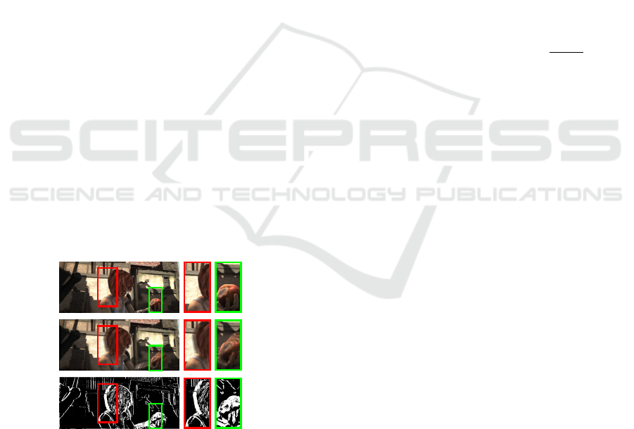
Figure 1 shows an example using the eighth frame

of the Alley1 sequence from the Sintel dataset (Butler

et al., 2012). The ﬁrst row shows the central image

while the second row depicts the denoised one. The

latter has been obtained according to the trajectories

described by the ground truths. The red and green

rectangles makes zoom in some regions from the re-

sults of the ﬁrst column.

Comparing both images, we observe a “halo ef-

fect” in the denoised image. This typically occurs

in occluded regions, where it is not possible to ﬁnd

the corresponding pixels in all the frames. The image

mask on the the third row represents the pixels where

the color difference is higher than a given threshold.

Here, it is easy to observe the occluded regions as well

as other regions affected by other effects.

Figure 1: Alley1 and its denoised image. The ﬁrst column

shows the central frame, the denoised image without dis-

carding pixels and the image mask. The second and third

columns show several details of the images at the ﬁrst col-

umn. The “halo effect” appears in the occluded regions,

which are detected on the mask.

In our experimental framework, the original se-

quences are randomly disturbed by adding white

Gaussian noise (AWGN) according to a known stan-

dard deviation, σ. We discard the pixels for which

the quadratic difference between the original and the

warped images are bigger than 2 · σ

. In these cases,

the noisy pixels are used for the ﬁnal result and the

image mask is activated in those positions as in the

last column of Fig. 1.

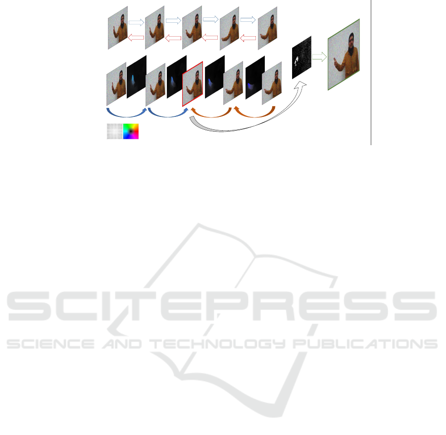
Figure 2 shows a diagram of the framework. The

denoised image is calculated as an average of the

color values in each pixel. Additionally, we esti-

mate an error function as the difference between the

denoised values and the pixels in the central image.

This allows us to detect pixels that suffer from oc-

clusions or brightness changes, or that are not cor-

rectly matched by the optical ﬂow method. Finally,

we obtain the root mean square error (RMSE) and

peak signal-to-noise ratio (PSNR) between the de-

noised and the original clean image.

The video denoising framework also calculates

the RMSE

and PSNR

removing the pixels of the

mask, and the percentage of pixels (density) used in

the average. We also calculate the ratio between the

RMSE

and the density as RMSE

RMSE

density

3 EXPERIMENTS

We compare the performance of several optical ﬂow

methods for video denoising and also the results

given by the ground truth motions (GT). Our exper-

iments include the algorithms published in (Monz

et al., 2016; S

anchez et al., 2013; S

anchez et al.,

2013; Meinhardt-Llopis et al., 2013) of the original

methods (Monz

on et al., 2016; Brox et al., 2004;

Zach et al., 2007; Horn and Schunck, 1981), respec-

tively. We shall refer to them as RDPOF, ROF, TV-

L1 and HS, respectively. The method of S

anchez et

al. (S

anchez et al., 2013) and the temporal extension

of ROF are named as TCOF and ROF

. The standard

datasets only provide the forward optical ﬂows, so we

calculate the backward motions using the method pro-

posed in (S

anchez et al., 2015).

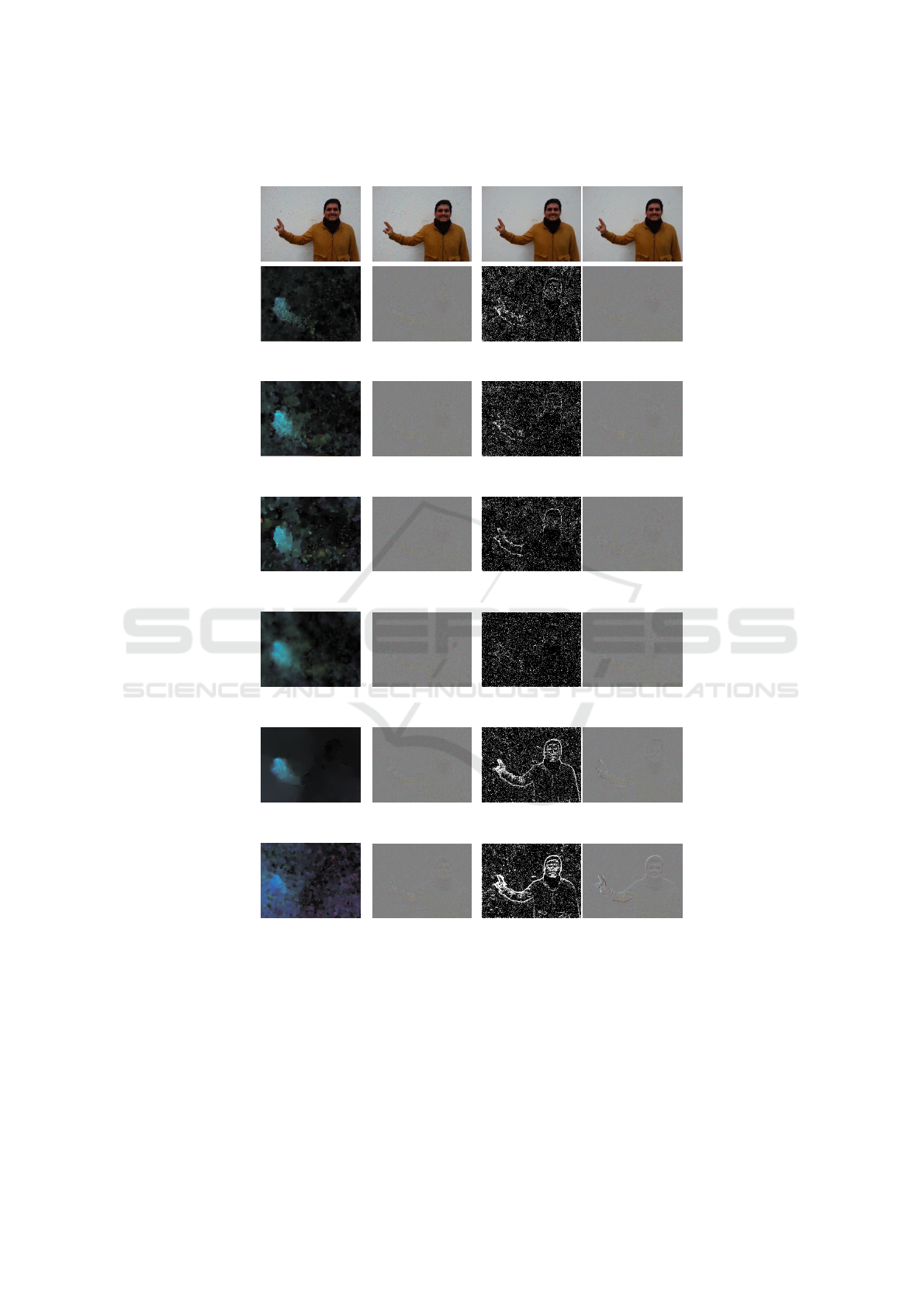
First, we compare the results for a given frame us-

ing the sequences of Alley1 (Fig. 3) and Bandage1

(Fig. 4) from the Sintel dataset. Figure 5 shows the

results from a video of a person moving his right arm.

The number of images of the sequences is 50 and the

size is 1024 × 436, while the Arm video contains 255

frames and its size is 320 × 240. The level of noise

introduced in these images is for σ = 10.

In each ﬁgure, the ﬁrst row contains two consec-

utive noisy frames, the original image and the best

denoised result. The following rows show the re-

sults using the ground truth, RDPOF, ROF, TV-L1,

HS, ROF

and TCOF, respectively. The ﬁrst col-

VISAPP 2020 - 15th International Conference on Computer Vision Theory and Applications

718

Compute Forward

and Backward Flows

Compute the average

using the mask

Warping

the

images

according

the

trajectories

Figure 2: Pipeline for video denoising: First, we add white Gaussian noise (AWGN) to the image sequence; second, the

optical ﬂow is calculated in both directions between consecutive frames; then, each image is denoised with the information of

several neighbor images; and, ﬁnally, we compute the root mean square error (RMSE) with respect to the original image. In

this ﬁgure, we illustrate an example with 2 frames in each direction.

umn depicts the calculated ﬂow from the central to

its successive frame. The second column shows the

error image between the original and the denoised im-

ages, taking into account the occlusion mask, which is

shown in the third column. The fourth one shows the

error image without using the mask. Below the im-

ages, we show the average angular error (AAE) and

the end-point error (EPE), that are standard metrics to

measure the optical ﬂow quality (Baker et al., 2007),

the parameters used, and the corresponding PSNR,

RMSE and density, in each case. In these experiments

we used 9 frames (n = 4).

Analyzing the results, we observe that the PSNR

and RMSE

using the masks are similar but the AAE

and EPE are very different. The RMSE difference be-

tween the ground truth and the other optical ﬂow re-

sults is around 5%, except for the temporal methods.

This means that they are equally good for denoising

purposes.

We also notice that, interestingly, the images cal-

culated without the masks achieve good results in

spite of the fact that the vector ﬁelds are clearly differ-

ent in several methods. For instance, the ﬂows found

for HS in Fig. 4 are evidently worse than those ob-

tained with the RDPOF and ROF methods. However,

the differences in the denoising results are not signif-

icant. The results for the ground truth are the worst

due to the halo effect produced at occlusions.

Table 1 shows the numerical results of the same

sequences but for the whole videos. The σ values are

10 and 50. It also includes the average of the runtime

required by the optical ﬂow methods. We write in

boldface the best RMSE for each sequence.

In general, the temporal methods provide the

higher errors and require the biggest execution times,

specially TCOF. On the other hand, the results con-

ﬁrm that the best optical ﬂows are not necessarily the

best for denoising. Furthermore, optical ﬂow ﬁelds

that are clearly worse compared to the ground truth,

are not so different for video denoising.

In our opinion, the most desired method for de-

noising is TV-L1, although its results are not always

the best. The error differences with respect to the

other alternatives are not signiﬁcant. Besides, if we

take into account the speed, this method is by far the

best choice.

4 CONCLUSION

In this work, we analyzed the inﬂuence of several op-

tical ﬂow methods for noise reduction. Experiments

prove that optical ﬂow is very useful but its accu-

racy is not as relevant as expected. We observed that

the methods yielding the best AAE and EPE are not

necessarily associated with the best denoising results.

This can be easily observed with the ground truth mo-

tion, where the denoised sequences are usually the

worst. Here it is important to distinguish between

optical ﬂow and motion estimation: The motion of

real scenes generates trajectories that do not neces-

sarily preserve the intensity of the pixels along the se-

quence, while the optical ﬂow ﬁnds correspondences

based on the similarity of the intensities. For this rea-

son, the results of such different strategies, like Horn

and Schunck or TV-L1, are very similar.

At the lights of our results, we may conclude that

the best strategy for video denoising is the TV-L1

method. This is not for the accuracy of its ﬂow ﬁelds

in general, but for its fast running times.

Comparison of the Optical Flow Quality for Video Denoising

719

Central frame

(σ = 10)

Successive frame

(σ = 10)

Original frame Denoised frame

PSNR

= 39.41

RMSE

= 2.72

Density = 73.47%

RMSE

= 3.71

PSNR= 31.72

RMSE= 6.60

RDPOF

AAE= 6.28, EPE= 0.47

α = 10, γ = 0

PSNR

= 38.76

RMSE

= 2.87

Density = 78.00%

RMSE

= 3.69

PSNR= 37.73

RMSE= 3.31

ROF

AAE= 7.68, EPE= 0.48

α = 5, γ = 1

PSNR

= 38.87

RMSE

= 2.90

Density = 76.65%

RMSE

= 3.67

PSNR= 37.63

RMSE= 3.34

TV-L1

AAE= 7.09, EPE= 0.45

λ = 0.3

PSNR

= 38.47

RMSE

= 2.84

Density = 78.48%

RMSE

= 3.62

PSNR= 37.70

RMSE= 3.32

AAE= 11.00, EPE= 0.66

α = 25

PSNR

= 38.88

RMSE

= 2.89

Density = 76.17%

RMSE

= 3.80

PSNR= 37.03

RMSE= 3.58

ROF

AAE= 6.42, EPE= 0.56

α = 25, γ = 1

PSNR

= 39.21

RMSE

= 2.78

Density = 72.31%

RMSE

= 4.02

PSNR= 35.33

RMSE= 4.36

TCOF

AAE= 18.57,EPE= 1.11

α = 10, δ = 0.1

γ = 10, β = 0.1

PSNR

= 38.35

RMSE

= 3.08

Density = 61.59%

RMSE

= 5.00

PSNR= 32.46

RMSE= 6.07

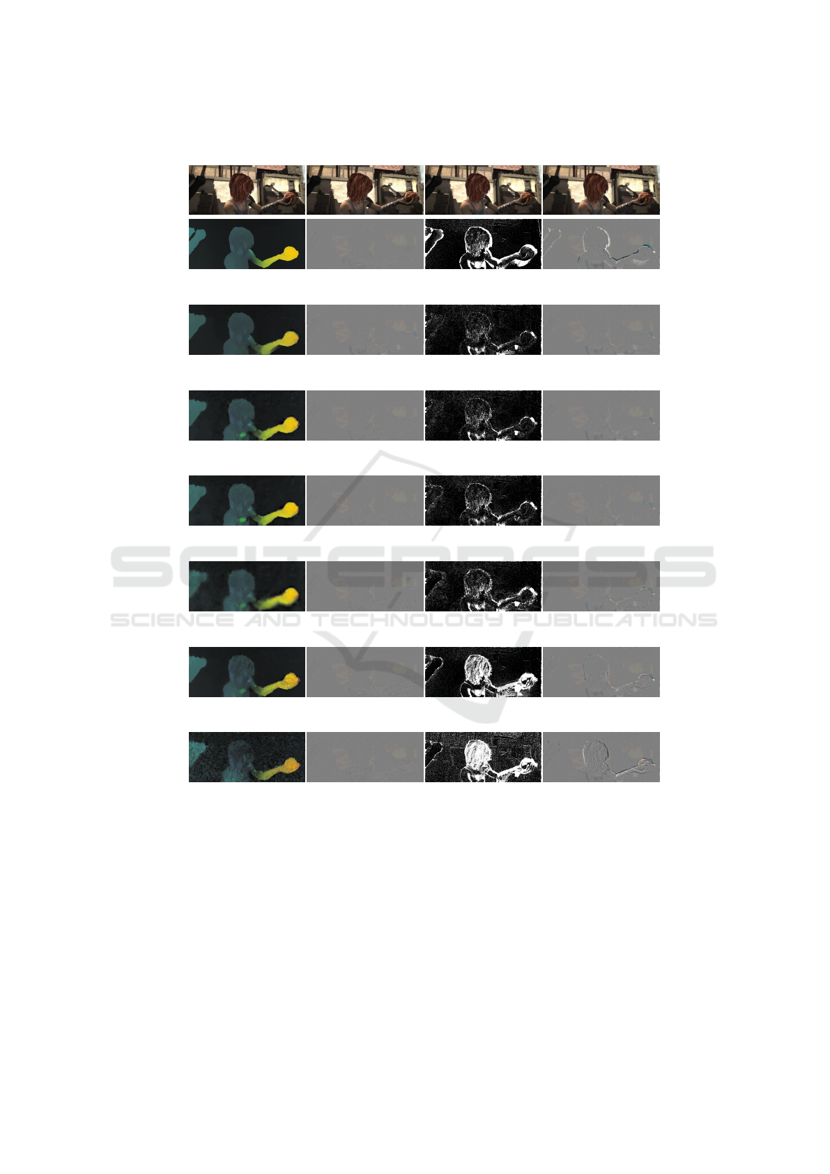
Figure 3: Denoising results for the Alley1 sequence. In the ﬁrst row, two images of the Alley1 sequence with Gaussian noise

of σ = 10, the original image, and the denoised result are shown. In the second row, we show the ground truth (GT) motion,

the error image between the original frame and the denoised result using the mask (third column), and the error image without

the mask. The rest of rows correspond to the results of the RDPOF, ROF, TV-L1, HS, ROF

and TCOF methods, respectively.

See the text for more explanations.

ACKNOWLEDGEMENTS

This work has been partly ﬁnanced by Ofﬁce of

Naval research grant N00014-17-1-2552, DGA Astrid

project “ﬁlmer la Terre” n

ANR-17-ASTR-0013-01,

DGA Defals challenge n

ANR-16-DEFA-0004-01.

Special thanks to Prof. Jean-Michel Morel for his

guidance and help during this research work.

VISAPP 2020 - 15th International Conference on Computer Vision Theory and Applications

720

Central frame

(σ = 10)

Successive frame

(σ = 10)

Original frame Denoised frame

PSNR

= 38.38

RMSE

= 3.07

Density = 48.55%

RMSE

= 6.32

PSNR= 29.50

RMSE= 8.53

RDPOF

AAE= 13.52, EPE= 0.53

α = 5, γ = 0

PSNR

= 38.30

RMSE

= 3.10

Density = 69.76%

RMSE

= 4.44

PSNR= 36.74

RMSE= 3.71

ROF

AAE= 15.37, EPE= 0.57

α = 5, γ = 1

PSNR

= 38.44

RMSE

= 3.04

Density = 70.23%

RMSE

= 4.33

PSNR= 36.74

RMSE= 3.71

TV-L1

AAE= 21.68, EPE= 0.76

λ = 0.3

PSNR

= 38.78

RMSE

= 2.95

Density = 73.35%

RMSE

= 4.03

PSNR= 36.50

RMSE= 3.84

AAE= 26.16, EPE= 1.06

α = 10

PSNR

= 38.45

RMSE

= 3.04

Density = 73.31%

RMSE

= 4.15

PSNR= 36.30

RMSE= 3.90

ROF

AAE= 12.65, EPE= 0.52

α = 5, γ = 0

PSNR

= 38.85

RMSE

= 2.91

Density = 62.25%

RMSE

= 4.67

PSNR= 34.56

RMSE= 4.76

TCOF

AAE= 21.74, EPE= 0.84

α = 50, δ = 0.01

γ = 10,, β = 0

PSNR

= 38.73

RMSE

= 2.94

Density = 61.74%

RMSE

= 4.77

PSNR= 33.63

RMSE= 5.30

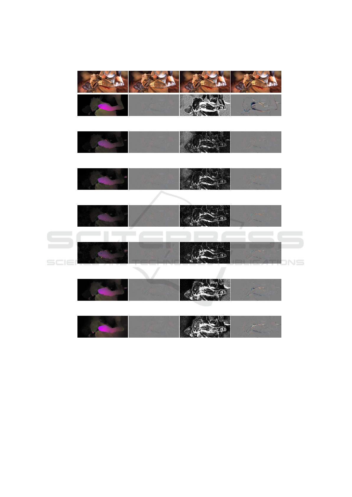
Figure 4: Denoising results for the Bandage1 sequence. In the ﬁrst row, two images of the Bandage1 sequence with Gaussian

noise of σ = 10, the original image, and the denoised result are shown. In the second row, we show the ground truth (GT)

motion, the error image between the original frame and the denoised result using the mask (third column), and the error image

without the mask. The rest of rows correspond to the results of the RDPOF, ROF, TV-L1, HS, ROF

and TCOF methods,

respectively. See the text for more explanations.

Comparison of the Optical Flow Quality for Video Denoising

721

Central frame

(σ = 10)

Successive frame

(σ = 10)

Central frame Denoised frame

RDPOF

α = 10, γ = 5

PSNR

= 38.62

RMSE

= 2.98

Density = 76.54%

RMSE

= 3.90

PSNR= 38.46

RMSE= 3.04

ROF

α = 10, γ = 5

PSNR

= 38.90

RMSE

= 2.89

Density = 78.09%

RMSE

= 3.70

PSNR= 38.38

RMSE= 3.07

TV-L1

λ = 0.1

PSNR

= 38.99

RMSE

= 2.85

Density = 78.86%

RMSE

= 3.63

PSNR= 38.45

RMSE= 3.04

α = 10

PSNR

= 38.72

RMSE

= 2.95

Density = 79.83%

RMSE

= 3.69

PSNR= 38.39

RMSE= 2.97

ROF

α = 25, γ = 5

PSNR

= 38.93

RMSE

= 2.88

Density = 74.57%

RMSE

= 3.86

PSNR= 38.25

RMSE= 3.11

TCOF

α = 10, δ = 0.001

γ = 5, β = 0

PSNR

= 38.96

RMSE

= 2.87

Density = 72.86%

RMSE

= 3.94

PSNR= 36.38

RMSE= 3.86

Figure 5: Denoising results for the Arm sequence. In the ﬁrst row, two images of the Arm sequence with Gaussian noise of

σ = 10, the original image, and the denoised result are shown. In the second row, we show the ground truth (GT) motion, the

error image between the original frame and the denoised result using the mask (third column), and the error image without the

mask. The rest of rows correspond to the results of the RDPOF, ROF, TV-L1, HS, ROF

and TCOF methods, respectively.

See the text for more explanations.

VISAPP 2020 - 15th International Conference on Computer Vision Theory and Applications

722

Table 1: Best AAE, EPE, average runtime to obtain the optical ﬂows, RMSE, RMSE

and densities (%) found for the

complete videos of Alley1, Bandage1 and the Arm sequence. The noise values are σ = 10 and σ = 50.

Alley1

(σ = 10)

Alley1

(σ = 50)

Bandage1

(σ = 10)

Bandage1

(σ = 50)

Arm

(σ = 10)

Arm

(σ = 50)

RMSE 7.60 16.07 8.53 18.50 - -

RMSE

2.89 14.16 3.24 15.21 - -

Densities 70.14% 81.69% 41.96% 68.10% - -

RDPOF

AAE 7.82

14.23

15.80

29.48

- -

EPE 0.61 1.11 1.23 1.89 - -

Time 3.6(s) 3.85(s) 3.57(s) 3.87(s) 0.6(s) 0.8(s)

RMSE 3.73 15.25 4.15 15.09 3.13 14.12

RMSE

3.05 14.77 3.26 14.69 3.00 13.85

Densities 77.37% 83.89% 65.91% 84.08% 76.31% 83.51%

ROF

AAE 7.51

10.76

16.01

26.68

- -

EPE 0.60 0.94 1.20 1.64 - -

Time 5.43(s) 6.39(s) 5.67(s) 6.39(s) 1.6(s) 2(s)

RMSE 3.77 14.80 4.34 14.96 3.11 13.93

RMSE

3.02 14.30 3.21 14.53 2.91 13.81

Densities 76.65% 83.75% 64.52% 83.50% 77.15% 84.81%

TV-L1

AAE 7.02

14.48

21.69

28.64

- -

EPE 0.58 0.99 2.11 1.69 - -

Time 2(s) 2.6(s) 2(s) 2.2(s) 0.25(s) 0.21(s)

RMSE 3.87 14.78 4.44 14.94 3.09 13.77

RMSE

2.96 14.37 3.11 14.48 2.88 13.72

Densities 75.67% 84.12% 69.27% 83.58% 78.16% 84.91%

AAE 9.91

21.12

22.15

33.53

- -

EPE 0.75 1.31 1.43 2.04 - -

Time 4.8(s) 6.5(s) 6.51(s) 4.83(s) 5.35(s) 5.86(s)

RMSE 4.26 14.98 4.84 15.23 3.07 13.98

RMSE

3.00 14.53 3.16 14.70 2.96 13.76

Densities 73.97% 84.10% 68.14% 83.38% 79.83% 84.62%

ROF

AAE 6.81

12.11

15.87

26.41

- -

EPE 0.64 0.94 1.41 1.77 - -

Time 6.9(s) 7.47(s) 7.32(s) 7.68(s) 1.23(s) 1.82(s)

RMSE 5.33 15.1 6.58 15.72 3.39 14.02

RMSE

2.91 14.43 3.14 14.72 2.91 13.71

Densities 70.40% 83.31% 52.41% 81.27% 75.26% 83.28%

TCOF

AAE 19.80

24.33

27.62

30.45

- -

EPE 1.26 1.72 2.25 2.83 - -

Time 88.52(s) 75.52(s) 79.18(s) 52.12(s) 14.27(s) 10.18(s)

RMSE 5.75 15.95 8.55 16.60 3.55 14.28

RMSE

3.18 15.01 3.05 15.24 2.88 13.90

Densities 65.06% 82.39% 45.75% 79.83% 74.19% 83.87%

REFERENCES

Arias, P. and Morel, J.-M. (2018). Video denois-

ing via empirical bayesian estimation of space-time

patches. Journal of Mathematical Imaging and Vision,

60(1):70–93.

Baker, S., Scharstein, D., Lewis, J., Roth, S., Black, M.,

and Szeliski, R. (2007). A database and evaluation

methodology for optical ﬂow. In International Con-

ference on Computer Vision (ICCV 2007).

Boulanger, J., Kervrann, C., and Bouthemy, P. (2007).

Space-time adaptation for patch-based image se-

quence restoration. IEEE Transactions on Pattern

Analysis and Machine Intelligence, 29(6):1096–1102.

Brox, T., Bruhn, A., Papenberg, N., and Weickert, J. (2004).

High accuracy optical ﬂow estimation based on a the-

Comparison of the Optical Flow Quality for Video Denoising

723

ory for warping. In Pajdla, T. and Matas, J., editors,

European Conference on Computer Vision (ECCV),

volume 3024 of LNCS, pages 25–36, Prague, Czech

Republic. Springer.

Buades, A., Lisani, J., and Miladinovi

c, M. (2016). Patch-

based video denoising with optical ﬂow estimation.

IEEE Transactions on Image Processing, 25(6):2573–

2586.

Butler, D. J., Wulff, J., Stanley, G. B., and Black, M. J.

(2012). A naturalistic open source movie for optical

ﬂow evaluation. In A. Fitzgibbon et al. (Eds.), editor,

European Conf. on Computer Vision (ECCV), Part IV,

LNCS 7577, pages 611–625. Springer-Verlag.

Ehret, T., Morel, J., and Arias, P. (2018). Non-local kalman:

A recursive video denoising algorithm. In 2018 25th

IEEE International Conference on Image Processing

(ICIP), pages 3204–3208.

Horn, B. and Schunck, B. (1981). Determining optical ﬂow.

MIT Artiﬁcial Intelligence Laboratory, 17:185–203.

Larsson, M. and S

oderstr

om, L. (2015). Analysis of optical

ﬂow algorithms for denoising. Student Paper.

Liu, C. and Freeman, W. T. (2010). A high-quality video

denoising algorithm based on reliable motion estima-

tion. In Daniilidis, K., Maragos, P., and Paragios, N.,

editors, Computer Vision – ECCV 2010, pages 706–

719, Berlin, Heidelberg. Springer Berlin Heidelberg.

Lucas, B. D. and Kanade, T. (1981). An iterative image

registration technique with an application to stereo vi-

sion. In Proceedings of the 7th international joint

conference on Artiﬁcial intelligence - Volume 2, pages

674–679, San Francisco, CA, USA. Morgan Kauf-

mann Publishers Inc.

Meinhardt-Llopis, E., S

anchez, J., and Kondermann, D.

(2013). Horn-Schunck Optical Flow with a Multi-

Scale Strategy. Image Processing On Line, 3:151–

172.

Monz

on, N., Salgado, A., and S

anchez, J. (2016). Regular-

ization strategies for discontinuity-preserving optical

ﬂow methods. IEEE Transactions on Image Process-

ing, 25(4):1580–1591.

Monz

on, N., Salgado, A., and S

anchez, J. (2016). Robust

Discontinuity Preserving Optical Flow Methods. Im-

age Processing On Line, 6:165–182.

anchez, J., Meinhardt-Llopis, E., and Facciolo, G. (2013).

TV-L1 Optical Flow Estimation. Image Processing

On Line, 3:137–150.

anchez, J., Monz

on, N., and Salgado, A. (2013). Ro-

bust optical ﬂow estimation. Image Processing

On Line, 2013:252–270. http://dx.doi.org/10.

5201/ipol.2013.21.

anchez, J., Salgado, A., and Monz

on, N. (2013). Op-

tical ﬂow estimation with consistent spatio-temporal

coherence models. In International Conference on

Computer Vision Theory and Applications (VISAPP),

pages 366–370. Institute for Systems and Technolo-

gies of Information, Control and Communication.

anchez, J., Salgado, A., and Monz

on, N. (2015). Comput-

ing inverse optical ﬂow. Pattern Recognition Letters,

52:32 – 39.

Scharr, H. and Spies, H. (2005). Accurate optical ﬂow in

noisy image sequences using ﬂow adapted anisotropic

diffusion. Sig. Proc.: Image Comm., 20:537–553.

Sellent, A., Kondermann, D., Simon, S. J., Baker, S.,

Dedeoglu, G., Erdler, O., Parsonage, P., Unger, C.,

and Niehsen, W. (2012). Optical ﬂow estimation ver-

sus motion estimation.

Spies, H. and Scharr, H. (2001). Accurate optical ﬂow in

noisy image sequences. In Proceedings Eighth IEEE

International Conference on Computer Vision. ICCV

2001, volume 1, pages 587–592 vol.1.

Verri, A. and Poggio, T. A. (1989). Motion ﬁeld and opti-

cal ﬂow: Qualitative properties. IEEE Trans. Pattern

Anal. Mach. Intell., 11:490–498.

Zach, C., Pock, T., and Bischof, H. (2007). A Duality

Based Approach for Realtime TV-L1 Optical Flow.

In Hamprecht, F. A., Schn

orr, C., and J

ahne, B., ed-

itors, Pattern Recognition, volume 4713 of Lecture

Notes in Computer Science, chapter 22, pages 214–

223. Springer Berlin Heidelberg, Berlin, Heidelberg.

VISAPP 2020 - 15th International Conference on Computer Vision Theory and Applications

724