
An Inverse Method of the Natural Setting for Integer, Half-integer and
Rational “Perfect” Hypocycloids
Zarema S. Seidametova
1 a
and Valerii A. Temnenko
2 b
1
Crimean Engineering and Pedagogical University, 8 Uchebnyi Ln., Simferopol, 95015, Ukraine
2
Independent researcher, Simferopol, Ukraine
Keywords:
Hypocycloid, Perfect Hypocycloid, Inverse Method of Natural Setting for Planar Curves.
Abstract:
The paper describes a family of remarkable curves (integer and half-integer hypocycloids and rational perfect
hypocycloids) given in an inverse-natural form using a simple trigonometric relation s = s(χ), where s is the
arc coordinate and χ is the angle defining the direction of the tangent. In the paper we presented all perfect
hypocycloids with the number of cusps ν ≤ 10. From designing the hypocycloid using inverse natural setting
easy to determine the number of cusps and find the values of the λ
m
parameter, corresponding to perfect
hypocycloids.
1 INTRODUCTION
Many remarkable curves have emerged in mathemat-
ics over the past centuries. The study of these curves
is a very effective tool in the teaching of calculus, dif-
ferential geometry and computer science. Many great
curves are described in the classical book “A Catalog
of Special Plane Curves” (Lawrence, 2014) that fea-
tured more than 60 special curves. The other work on
plane curves is “A handbook on curves and their prop-
erties” (Yates, 2012). This handbook contains curves
constructions, equations, physical and mathematical
properties, and connections to each other.
Wang et al. (Wang et al., 2019) explored hypocy-
cloid’s parametric equation and discussed the appli-
cation of the astroid on the bus door for saving space.
For simulating its dynamic opening process, they used
MATLAB. There are a lot of examples of the using
curves and surfaces innovation in the architectural de-
signs of modern buildings (Biran, 2018).
Almost all curves can be represented mathemati-
cally and on a computer. The mathematical study of
curves and surfaces in space is called “differential ge-
ometry”. There are a lot of mathematical tools avail-
able to the computer scientist. The combination of
these tools depends on what and how curves need to
be represented.
There are different types of curves using in the
a
https://orcid.org/0000-0001-7643-6386
b
https://orcid.org/0000-0002-9355-9086
design of geometric data structures. For example,
Space-Filling Curves described in the papers (Asano
et al., 1997; Rad and Karimipour, 2019).
There are a lot of ways to define curves. One of
the most convenient ways to describe a plane curve is
the “Euler” or “natural” way of locally defining the
curve. In this method, the angle of inclination of the
tangent is set as a function of the length of the arc
along the curve.
In some situations, the “reverse” method of “nat-
ural” curve definition is convenient, in which the arc
length is set as a function of the angle of inclination of
the tangent. We will demonstrate in this article how
convenient this “reverse” method is when describing
some types of hypocycloids.
2 AN INVERSE METHOD OF THE
NATURAL SETTING FOR
PLANAR CURVES
One well known way to define flat curves is to de-
scribe them in the so-called natural form (or, another
name is “Euler’s form”):
χ = χ(s), (1)
where χ is an angle between some fixed direction – for
example, the x-axis – and the direction of the tangent
to the curve; s is the arc coordinate along the curve.
584
Seidametova, Z. and Temnenko, V.
An Inverse Method of the Natural Setting for Integer, Half-integer and Rational "Perfect" Hypocycloids.
DOI: 10.5220/0011009700003364
In Proceedings of the 1st Symposium on Advances in Educational Technology (AET 2020) - Volume 2, pages 584-589
ISBN: 978-989-758-558-6
Copyright
c
2022 by SCITEPRESS – Science and Technology Publications, Lda. All rights reserved

If the natural equation of the curve (1) is known,
then the equations of the corresponding curve in para-
metric form x = x(s), y = y(s) can be written in the
following form:
x =
s
Z
0
cosχ(s)ds + x
0
,
y =
s
Z
0
sinχ(s)ds + y
0
,
(2)
where (x
0
,y
0
) is an arbitrarily chosen point (x, y) in
the plane, corresponding on the curve to the origin of
the arc coordinate s = 0.
Leonhard Euler studied a family of curves of the
form (1) with a power-law dependence of χ on s
(χ = λs
p
, λ = const, p = const) (MacTutor History
of Mathematics, 2020). Euler called these curves as
“clothoids”. The most famous of these curves for p=2
is called the “Euler spiral” or “Cornu spiral”. Euler in-
vestigated this curve a century earlier than did Marie
Alfred Cornu.
Instead of the equation (1), we can consider the
inverse method of natural setting for the curve:
s = s(χ). (3)
This method is convenient if the function inverse
to (3) is multivalued or does not have an explicit ana-
lytic expression.
Equations (2) with this method for specifying the
curve (3) become:
x(χ) =
χ
Z
0
cosχ ·
ds
dχ
dχ + x
0
,
y(χ) =
χ
Z
0
sinχ ·
ds
dχ
dχ + y
0
.
(4)
Equations (4) define a parametric description of
the curve. In this specification parameter χ has clear
geometric meaning: it is the angle between the axis x
and the direction tangent to the curve.
3 INTEGER HYPOCYCLOIDS
We consider in this note a one-parameter family of
curves of the form (3):
s =
n
2
− 1
n
2
· sin(nχ), (5)
in which n ≥ 2 is an integer parameter. Let’s call the
equation (5) the “trigonometric Euler relation”. This
relation in local variables (s,λ) describes the classic
family of curves: integer hypocycloids.
For an even value of n, the range of the function
(5) is 0 ≤ χ ≤ 2π. For an odd value of n, the range
of the function (5) is 0 ≤ χ ≤ π. On this interval
the trigonometric Euler’s relation (5) defines a closed
curve.
Assuming that x
0
= 0, y
0
= 1/n, and performing
the integration in (4), we obtain the equations of the
integer hypocycloids in parametric form:
x =
1
2n
(n + 1) sin
(n − 1) χ
+
(n − 1) sin
(n + 1) χ
,
y =
1
2n
(n + 1) cos
(n − 1) χ
−
(n − 1) cos
(n + 1) χ
.
(6)
4 CUSPS OF THE INTEGER
HYPOCYCLOIDS
The curves (6) are smooth everywhere except the
points χ
n,k
, in which the cusps of the curve (6) are
located. The positions of the cusps’ vertices are de-
termined by the points of a curvature singularity of
the curve (6):
χ
0
s
=
1
s
0
χ
=
n
(n
2
− 1)cos(nχ)
. (7)
Respectively, the cusp-points are zeros of cos(nχ):
χ
n,k
=
π
2n
(2k +1). (8)
Let ν denote a number of cusps for the integer
hypocycloids (6). In equation (8) k can take 2n val-
ues for even n (0 ≤ k ≤ 2n − 1) and n values for odd
(0 ≤ k ≤ n − 1). Accordingly, the integer hypocy-
cloids can have an odd number of ν cusps at n =
2m + 1 or the it can have ν as a multiple of 4 (ν = 4m
at n = 2m). There is no integer hypocycloids with
ν = 4m + 2 cusps – for example, there is no six-
pointed “Euler star”, but there is a five-pointed Euler
star, eight-pointed and twelve-pointed Euler stars.
Substituting (8) into (6), we define the positions
of the cusps’ vertices on the plane (x,y):
x
n,k
= (−1)
k
cos
π
2n
(2k +1)
,
y
n,k
= (−1)
k
sin
π
2n
(2k +1)
.
(9)
All the cusps’ vertices (9) lie on a circle of unit
radius with the center at the origin.
An Inverse Method of the Natural Setting for Integer, Half-integer and Rational "Perfect" Hypocycloids
585
5 APPEARANCE OF THE
INTEGER HYPOCYCLOIDS
Figures 1-5 show an appearance of the integer
hypocycloids with the number of rays ν, equal to 3,
4, 5, 8 and 12.
-1.0 -0.5 0.0 0.5 1.0
-1.0
-0.5
0.0
0.5
1.0
X
Y
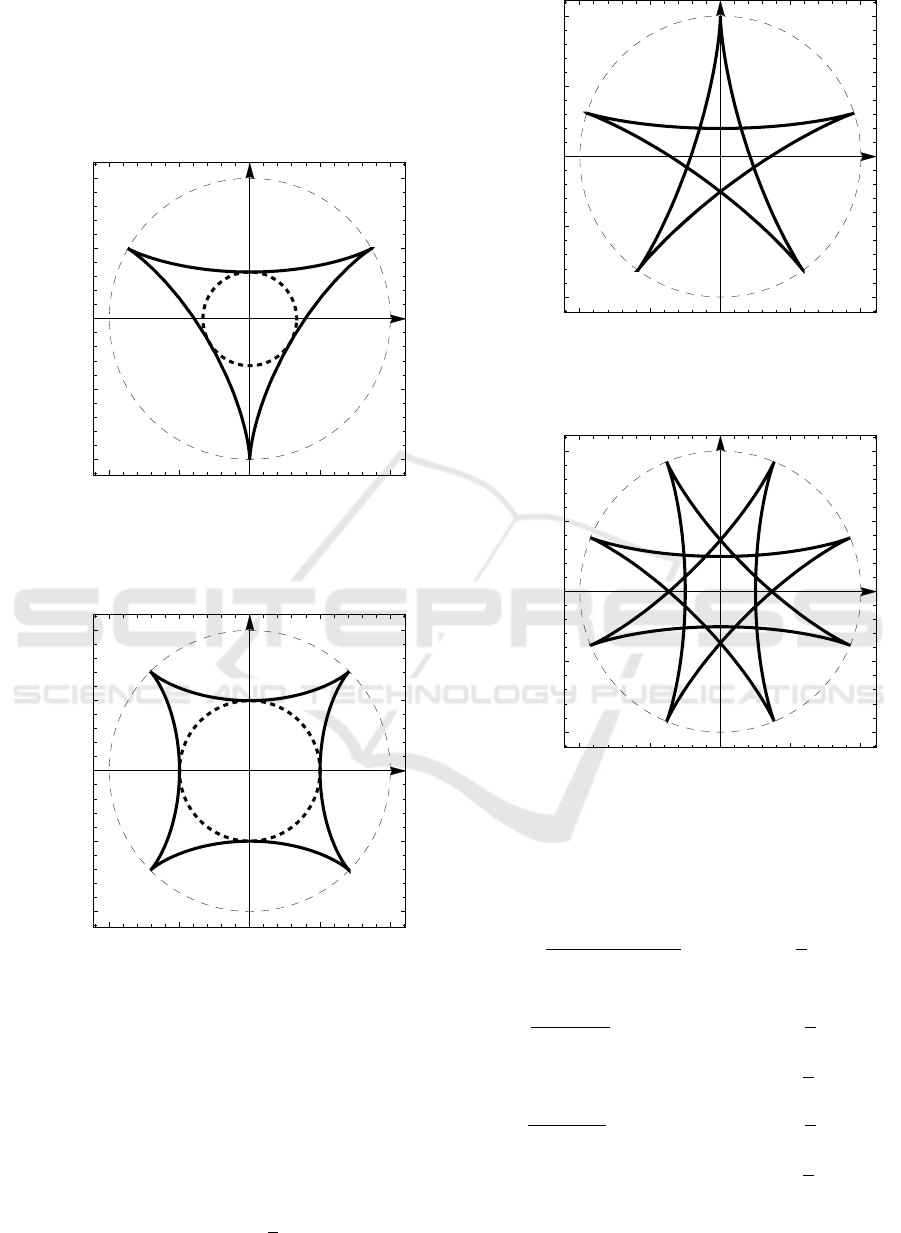
Figure 1: The tricuspidate hypocycloid (deltoid) (n = 3,
ν = 3).
-1.0 -0.5 0.0 0.5 1.0
-1.0
-0.5
0.0
0.5
1.0
X
Y
Figure 2: The tetracuspidate hypocycloid (astroid) (n = 2,
ν = 4).
6 HALF-INTEGER
HYPOCYCLOIDS
Consider the half-integer hypocycloid, assuming that
in equations (5) and (6) the integer parameter n is re-
placed by a half-integer n → n +
1
2
(n ≥ 1).
-1.0 -0.5 0.0 0.5 1.0
-1.0
-0.5
0.0
0.5
1.0
X
Y
Figure 3: The pentacuspidate hypocycloid (the integer
hypocycloid with n = 5, ν = 5).
-1.0 -0.5 0.0 0.5 1.0
-1.0
-0.5
0.0
0.5
1.0
X
Y
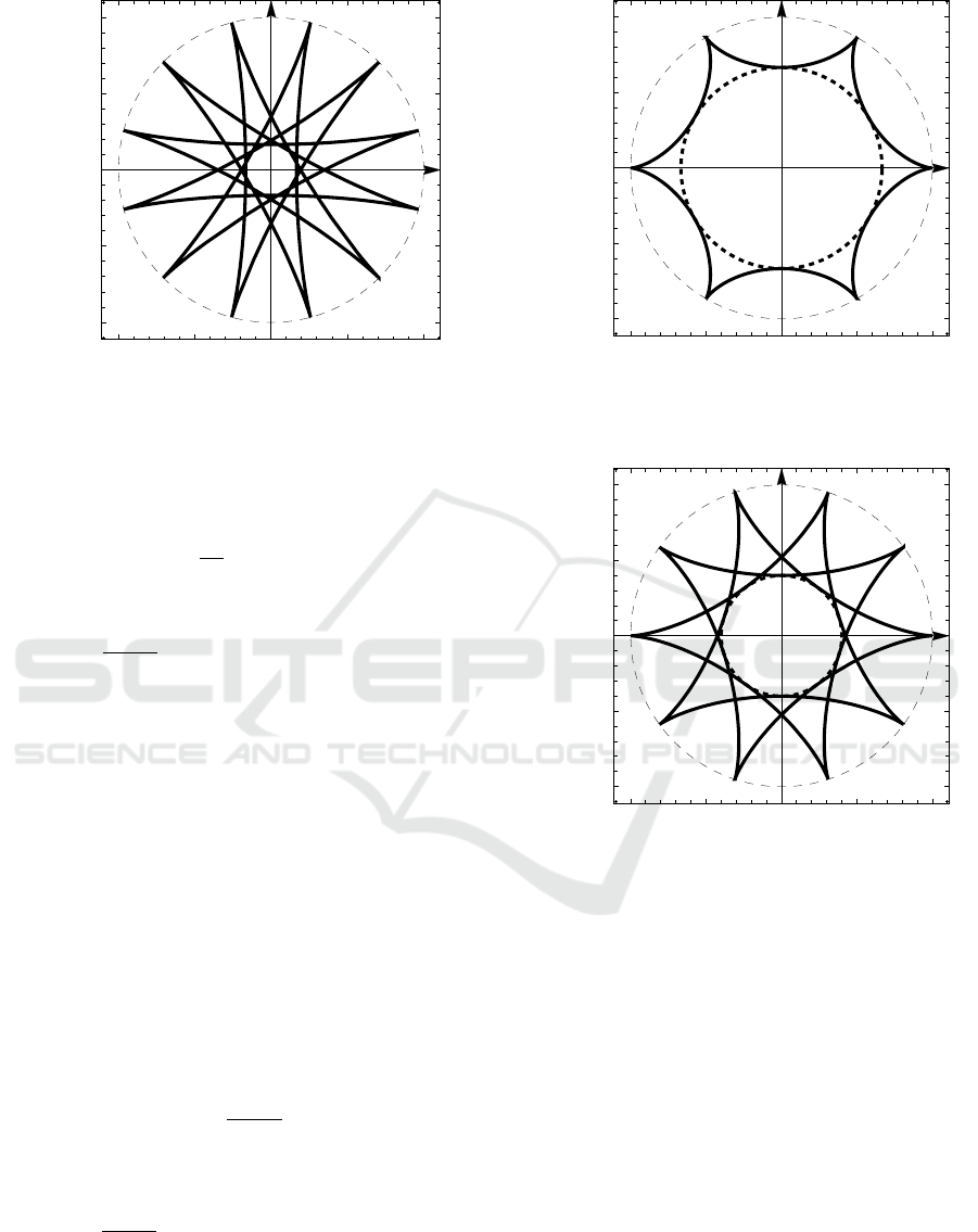
Figure 4: The octacuspidate hypocycloid (the integer
hypocycloid with n = 4, ν = 8).
With half-integer parameter, the hypocycloid
equations (5) and (6) take the following form:
s =
(2n − 1) (2n + 3)
(2n + 1)
2
sin
(2n + 1)
χ
2
, (10)
x =
1
2(2n + 1)
(2n + 3) sin
(2n − 1)
χ
2
+
+(2n − 1)sin
(2n + 3)
χ
2
,
y =
1
2(2n + 1)
(2n + 3) cos
(2n − 1)
χ
2
−
− (2n − 1)cos
(2n + 3)
χ
2
.
(11)
The functions x(χ) and y(χ) (11) are periodic in
the argument χ with a period P = 4π.
AET 2020 - Symposium on Advances in Educational Technology
586
-1.0 -0.5 0.0 0.5 1.0
-1.0
-0.5
0.0
0.5
1.0
X
Y
Figure 5: The dodecacuspidate hypocycloid (the integer
hypocycloid with n = 6, ν = 12).
The positions of the cusps of the half-integer
hypocycloid (11) are determined by the condition:
ds
dχ
= 0, (12)
or
χ
k
= π
2k +1
2n + 1
; 0 ≤ k ≤ k
max
= 4n + 1. (13)
The number of cusps ν is determined by the con-
dition
ν = 1 + k
max
= 4n + 2. (14)
In accordance with (14), half-integer hypocy-
cloids together with integer hypocycloids make it pos-
sible to obtain an hypocycloid with any number of
rays. In particular, for n = 1, equation (1) describes a
six-beam astroid.
Figure 6 and figure 7 show half-integer hypocy-
cloids at n = 1 (figure 6) and n = 2 (figure 7).
A half-integer hypocycloid with n = 1 has no self-
intersection points (like two integer hypocycloids of
the lowest index 1, even and odd). The remain-
ing half-integer hypocycloids with n ≥ 2 (and integer
hypocycloids with index n ≥ 2) have self-intersection
points. The half-integer hypocycloids are located in
the ring between R
min
=
2
2n + 1
and R
max
= 1. It is
easy to show that these curves touch a circle of radius
R
min
in ν = 4n + 2 points for χ
t,k
:
χ
t,k
=
2πk
2n + 1
; 0 ≤ k ≤ k
max
= 4n + 1. (15)
The totality of integer and half-integer hypocy-
cloids forms the set of figures, called in (Seidametova
and Temnenko, 2019) “The Euler Insignia”.
-1.0 -0.5 0.0 0.5 1.0
-1.0
-0.5
0.0
0.5
1.0
X
Y
Figure 6: The half-integer hypocycloid at n = 1(the six-
pointed star).
-1.0 -0.5 0.0 0.5 1.0
-1.0
-0.5
0.0
0.5
1.0
X
Y
Figure 7: The half-integer hypocycloid at n = 2 (the ten-
pointed star).
7 THE PERFECT
HYPOCYCLOIDS
Let’s call a hypocycloid “perfect” if it has no self-
intersection points. An example of a perfect hypocy-
cloid is the deltoid (an odd integer hypocycloid with
n = 3 and ν = 3, figure 1), the astroid (an even inte-
ger hypocycloid, n = 2, ν = 4, figure 2) and the six-
point star (the half-integer hypocycloid, n = 1, ν = 6,
figure 6). All other integer and half-integer hypocy-
cloids, in particular, shown in figures 3, 4, 5, 7, are
not perfect.
Perfect hypocycloids are described by the trigono-
metric Euler relation (5), in which an integer n is re-
placed by some rational number λ
m
of a certain type.
The parameter λ
m
is an irreducible fraction of one of
An Inverse Method of the Natural Setting for Integer, Half-integer and Rational "Perfect" Hypocycloids
587
three possible types:
λ
m
=
2m + 1
2m − 1
; m ≥ 1. (16)
λ
m
=
2m
2m − 1
; m ≥ 1. (17)
λ
m
=
2m + 1
2m
; m ≥ 1. (18)
Let call perfect hypocycloids of the type (16)
the Odd-Odd perfect hypocycloids. Let call perfect
hypocycloids of the type (17) the Even-Odd perfect
hypocycloids. Let call perfect hypocycloids of the
type (18) the Odd- Even perfect hypocycloids. For
m = 1 a perfect hypocycloid of the type (16) is an
integer hypocycloid with three cusps (the deltoid, fig-
ure 1), a perfect hypocycloid of the type (17) is an
integer hypocycloid with four cusps (the astroid, fig-
ure 2), a perfect hypocycloid of the type (18) is a half-
integral six-pointed star (figure 6).
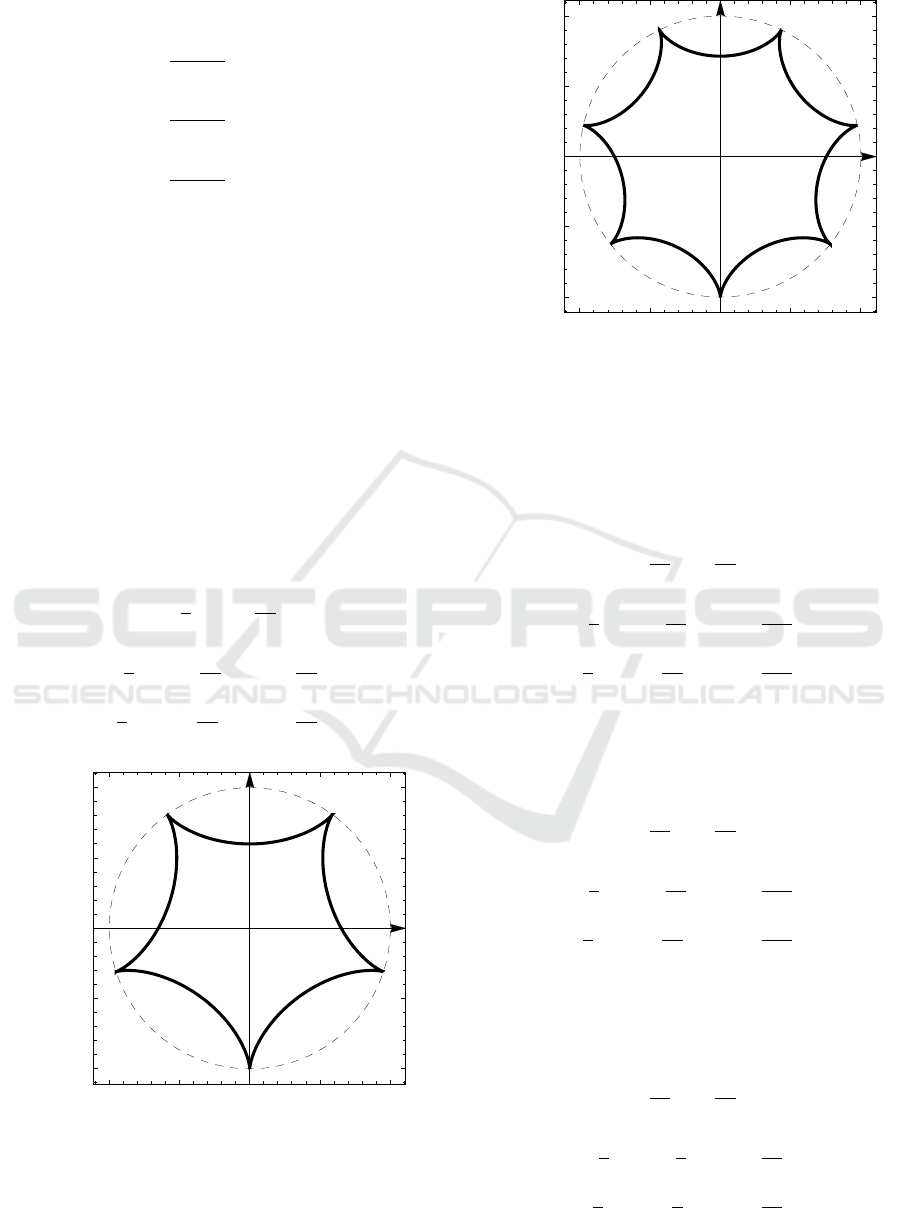
Figure 8 shows the Odd-Odd perfect hypocycloid
with m = 2 (the “five-pointed star of Euler”). In
accordance with relations (5) and (6) and the value
λ
m
= 5/3, the equations of this perfect hypocycloid
have the form:
s =
4
5
2
sin
5χ
3
, (19)
x =
1
5
4sin
2χ
3
+ sin
8χ
3
,
y =
1
5
4cos
2χ
3
− cos
8χ
3
.
(20)
-1.0 -0.5 0.0 0.5 1.0
-1.0
-0.5
0.0
0.5
1.0
X
Y
Figure 8: The Odd-Odd perfect hypocycloid with m = 2
(λ
m
= 5/3, the five-pointed star of Euler).
-1.0 -0.5 0.0 0.5 1.0
-1.0
-0.5
0.0
0.5
1.0
X
Y
Figure 9: The Odd-Odd perfect hypocycloid with m = 3
(λ
m
= 7/5, the seven-pointed star of Euler).
Figure 9 shows the Odd-Odd perfect hypocycloid
with m = 3 (λ
m
= 7/5, the “seven-pointed star of Eu-
ler”). The equations of this hypocycloid are follow-
ing:
s =
24
49
sin
7χ
5
, (21)
x =
1
7
6sin
2χ
5
+ sin
12χ
5
,
y =
1
7
6cos
2χ
5
− cos
12χ
5
.
(22)
Figure 10 shows the Odd-Odd perfect hypocy-
cloid with m = 4 (λ
m
= 9/7). This is the “nine-
pointed Euler star”). The equations of this curve are
following:
s =
32
81
sin
9χ
7
, (23)
x =
1
9
8sin
2χ
7
+ sin
16χ
7
,
y =
1
9
8cos
2χ
7
− cos
16χ
7
.
(24)
Figure 11 shows the Even-Odd perfect hypocy-
cloid with m = 2 (λ
m
= 4/3). This is the “eight-
pointed Euler star”). The equations of this curve are
following:
s =
7
16
sin
4χ
3
, (25)
x =
1
8
7sin
χ
3
+ sin
7χ
3
,
y =
1
8
7cos
χ
3
− cos
7χ
3
.
(26)
AET 2020 - Symposium on Advances in Educational Technology
588
-1.0 -0.5 0.0 0.5 1.0
-1.0
-0.5
0.0
0.5
1.0
X
Y
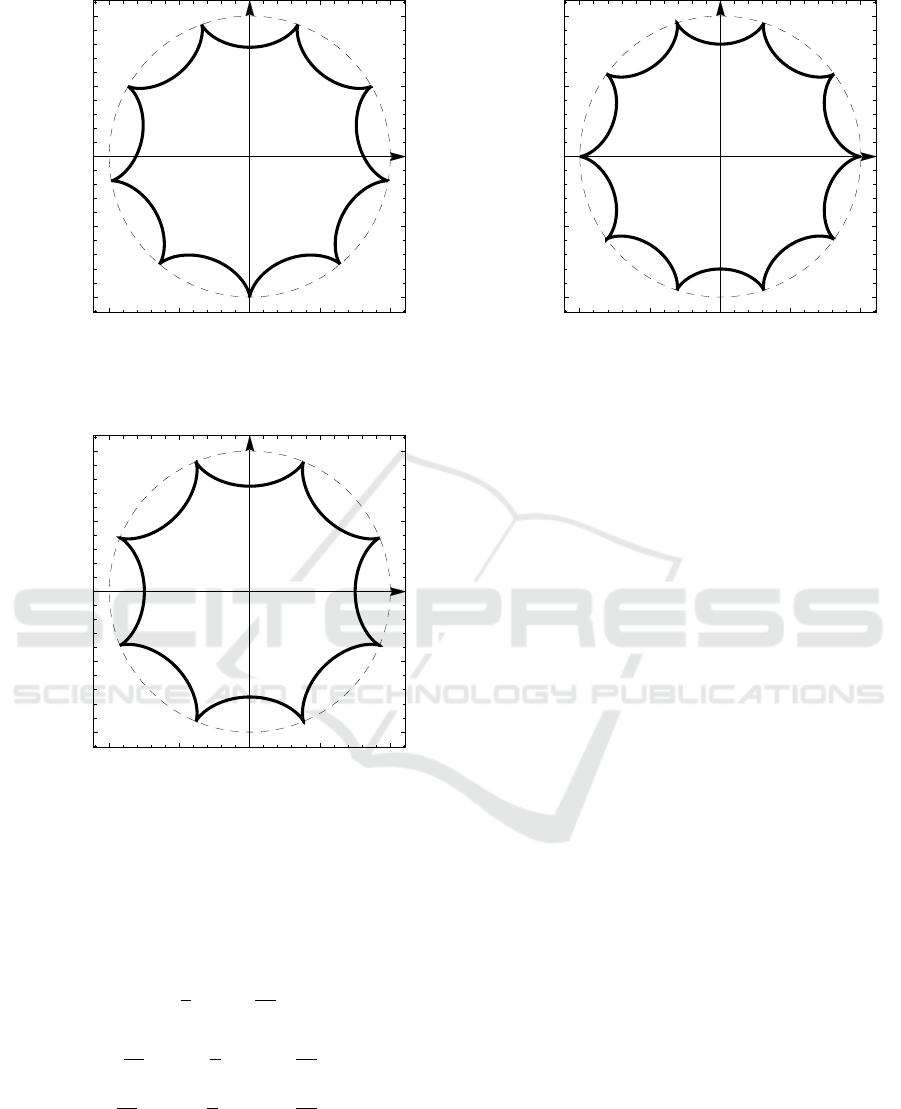
Figure 10: The Odd-Odd perfect hypocycloid with m = 4
(λ
m
= 9/7, the nine-pointed Euler star).
-1.0 -0.5 0.0 0.5 1.0
-1.0
-0.5
0.0
0.5
1.0
X
Y
Figure 11: The Even-Odd perfect hypocycloid with m = 2
(λ
m
= 4/3, the eight-pointed Euler star).
Figure 12 shows the Odd-Even perfect hypocy-
cloid with m = 2 (λ
m
= 5/4). This is the “ten-pointed
Euler star”). The equations of this curve are follow-
ing:
s =
3
5
2
sin
5χ
4
, (27)
x =
1
10
9sin
χ
4
+ sin
9χ
4
,
y =
1
10
9cos
χ
4
− cos
9χ
4
.
(28)
-1.0 -0.5 0.0 0.5 1.0
-1.0
-0.5
0.0
0.5
1.0
X
Y
Figure 12: The Odd-Even perfect hypocycloid with m = 2
(λ
m
= 5/4, the ten-pointed Euler star).
8 CONCLUSIONS
Figures 1, 2, 6, 8, 9, 10, 11, 12 presented in the paper
demonstrate all perfect hypocycloids with the number
of cusps ν ≤ 10.
Designing the hypocycloid by inverse natural set-
ting makes it easy to determine the number of cusps
and find the values of the λ
m
parameter ((16), (17) and
(18)), corresponding to perfect hypocycloids.
REFERENCES
Asano, T., Ranjan, D., Roos, T., Welzl, E., and Widmayer, P.
(1997). Space-filling curves and their use in the design
of geometric data structures. Theoretical Computer
Science, 181(1).
Biran, A. (2018). Geometry for Naval Architects.
Butterworth-Heinemann.
Lawrence, J. D. (2014). A Catalog of Special Plane Curves.
Dover Publications.
MacTutor History of Mathematics (2020). Famous Curves
Index. https://mathshistory.st-andrews.ac.uk/Curves/.
Rad, H. N. and Karimipour, F. (2019). Representation
and generation of space-filling curves: a higher-order
functional approach. Journal of Spatial Science.
Seidametova, Z. and Temnenko, V. (2019). Euler’s Insignia:
Some Admirable Curves Having a Simple Trigono-
metric Equation in a Natural Form. The College Math-
ematics Journal, 50(2).
Wang, B., Geng, Y., and Chu, J. (2019). Generation and
application of hypocycloid and astroid. Journal of
Physics: Conference Series, 1345(3):032085.
Yates, R. C. (2012). A Handbook On Curves And Their
Properties. Literary Licensing, LLC.
An Inverse Method of the Natural Setting for Integer, Half-integer and Rational "Perfect" Hypocycloids
589
