
Guessing Games Experiments in Ukraine: Learning towards
Equilibrium
Oleksii P. Ignatenko
1 a
1
Institute of Software Systems NAS Ukraine, 40 Academician Glushkov Ave., Kyiv, 03187, Ukraine
Keywords:
Behavioral Game Theory, Guessing Game, K-Beauty Contest, Active Learning, R.
Abstract:
The paper deals with experimental game theory and data analysis. The research question, formulated in this
work, is how players learn in complex strategic situations which they never faced before. We examine data
from different games, played during lectures about game theory and present findings about players progress
in learning while competing with other players. We proposed four “pick a number” games, all with similar-
looking rules but very different properties. These games were introduced (in the body of scientific popular
lectures) to very different groups of listeners. In this paper we present data gathered during lectures and
develop tool for exploratory analysis using R language. Finally, we discuss the findings propose hypothesis to
investigate and formulate open questions for future research.
1 INTRODUCTION
Game theory is a field of science which investigates
decision-making under uncertainty and interdepen-
dence, that is, when the actions of some players affect
the payoffs of others. Such situations arise around
us every day and we, consciously or unconsciously,
take part in them and try to succeed. The struggle to
achieve a better result (in some broad sense) is called
rationality. Every rational player must take into ac-
count the rules of the game, the interests and capabil-
ities of other participants in other words think strate-
gically. Game theory provides a tool for analyzing
such situations, which allows you to better understand
the causes of conflicts, learn to make decisions under
uncertainty, establish mutually beneficial cooperation
and much more.
A key element of strategic thinking is to include
into consideration what other agents do. Agent here is
a person, who can make decisions and his/her actions
have influence on the outcome. Naturally, person can-
not predict with 100% what will others do, so it is im-
portant to include into model beliefs about other per-
son thinking and update them during the game. Also,
if we can’t know what other player think, we can un-
derstand what is his/her best course of action. This is
the main research topic of game theory.
All this makes decision making very interesting
a
https://orcid.org/0000-0001-8692-2062
problem to investigate. In this work we will ap-
ply game theory to analyze such problems. Game
theory provides mathematical base for understanding
strategic interaction of rational players. There is im-
portant note about rationality, we should make. As
Robert Aumann formulate in his famous paper (Au-
mann, 1985), game theory operates with “homo ra-
tional”, ideal decision maker, who is able to define
his/her utility as a function and capable of computing
best strategy to maximize it. This is the main setup of
game theory and one of major lines of criticism. In re-
ality, of course, people are not purely rational in game
theory sense. They often do not want to concentrate
on a given situation to search for best decision or sim-
ply do not have enough time or capabilities for this.
Sometimes they just copycat behavior of others or use
some cultural codes to make strange decisions. Also
(as we see from the experiments) it seems that some-
times homo sapiens make decisions with reasons, one
can (with some liberty in formulation) label as “try
and see what happens”, “make random move and save
thinking energy” and even “make stupid move to spoil
game for others”.
This is rich area of research, where theoretical
constructions of game theory seems to fail to work
and experimental data shows unusual patterns. How-
ever, these patterns are persistent and usually do
not depend on age, education, country and other
things. During last 25 years behavioral game the-
ory in numerous studies examines bounded rational-
156
Ignatenko, O.
Guessing Games Experiments in Ukraine. Learning towards Equilibrium.
DOI: 10.5220/0010929600003364
In Proceedings of the 1st Symposium on Advances in Educational Technology (AET 2020) - Volume 2, pages 156-168
ISBN: 978-989-758-558-6
Copyright
c
2022 by SCITEPRESS – Science and Technology Publications, Lda. All rights reserved

ity (best close concept to rationality of game theory)
and heuristics people use to reason in strategic situa-
tions. For example we can note surveys of Crawford
et al.; Mauersberger and Nagel (Crawford et al., 2013;
Mauersberger and Nagel, 2018). Also there is com-
prehensive description of the field of behavioral game
theory by Camerer (Camerer, 2011).
Also we can note work of Gill and Prowse (Gill
and Prowse, 2016), where participants were tested on
cognitive abilities and character skills before the ex-
periments. Then authors perform statistical analysis
to understand the impact of such characteristics on the
quality of making strategic decisions (using p-beauty
contest game with multiple rounds). In more recent
work of Fe et al. (Fe et al., 2019) even more elabo-
rate experiments are presented. It is interesting that in
the mentioned paper experiments are very strict and
rigorous (as close to laboratory purity as possible) in
contrast to games, played in our research. But in the
end of the day the results are not differ very much.
The guessing games are notable part of research
because of their simplicity for players and easy anal-
ysis of rules from game theoretic prospective. In
this paper we present results of games played during
2018–2020 years in series of scientific popular lec-
tures. The audience of these lectures was quite hetero-
geneous, but we can distinguish three main groups:
• kids (strong mathematical schools, ordinary
schools, alternative education schools);
• students (bachelor and master levels);
• mixed adults with almost any background;
• businessmen;
• participants of Data Science School.
We propose framework of four different games,
each presenting one idea or concept of game theory.
These games were introduced to people with no prior
knowledge (at least in vast majority) about the the-
ory. From the other hand, games have simple formu-
lation and clear winning rules, which makes them in-
tuitively understandable even for kids. This makes
these games perfect choice to test ability of strate-
gic thinking and investigate process of understanding
of complex concepts during the play, with immediate
application to the game. This dual learning, as we
can name it, shows how players try-and-learn in real
conditions and react to challenges of interaction with
other strategic players.
1.1 Game Theory Definitions
We will consider games in strategic or normal form in
non-cooperative setup. A non-cooperativeness here
does not imply that the players do not cooperate, but
it means that any cooperation must be self-enforcing
without any coordination among the players. Strict
definition is as follows.
A non-cooperative game in strategic (or normal)
form is a triplet G = {N , {S
i
}
i=∈N
, {u
i
}
i∈N
},
where:
• N is a finite set of players, N = {1, . . . , N};
• S
i
is the set of admissible strategies for player i;
• u
i
: S −→ R is the utility (payoff) function for
player i, with S = {S
1
×·· ·×S
N
} (Cartesian prod-
uct of the strategy sets).
A game is said to be static if the players take their
actions only once, independently of each other. In
some sense, a static game is a game without any no-
tion of time, where no player has any knowledge of
the decisions taken by the other players. Even though,
in practice, the players may have made their strate-
gic choices at different points in time, a game would
still be considered static if no player has any informa-
tion on the decisions of others. In contrast, a dynamic
game is one where the players have some (full or im-
perfect) information about each others’ choices and
can act more than once.
Summarizing, these are games where time has a
central role in the decision-making. When dealing
with dynamic games, the choices of each player are
generally dependent on some available information.
There is a difference between the notion of an action
and a strategy. To avoid confusions, we will define a
strategy as a mapping from the information available
to a player to the action set of this player.
Based on the assumption that all players are ra-
tional, the players try to maximize their payoffs
when responding to other players’ strategies. Gen-
erally speaking, final result is determined by non-
cooperative maximization of integrated utility. In
this regard, the most accepted solution concept for a
non-cooperative game is that of a Nash equilibrium,
introduced by John F. Nash. Loosely speaking, a
Nash equilibrium is a state of a non-cooperative game
where no player can improve its utility by changing
its strategy, if the other players maintain their cur-
rent strategies. Of course players use also informa-
tion and beliefs about other players, so we can say,
that (in Nash equilibrium ) beliefs and incentives are
important to understand why players choose strategies
in real situations. Formally, when dealing with pure
strategies, i.e., deterministic choices by the players,
the Nash equilibrium is defined as follows:
A pure-strategy Nash equilibrium (NE) of a non-
cooperative game G is a strategy profile s
0
∈ S such
that for all i ∈ N we have the following inequality:
Guessing Games Experiments in Ukraine. Learning towards Equilibrium
157

u
i
(s
0
i
, s
0
−i
) ≥ u
i
(s
i
, s
0
−i
)
for all s
i
∈ S
i
.
Here s
−i
= {s
j
| j ∈ N , j 6= i} denotes the vector
of strategies of all players except i. In other words,
a strategy profile is a pure-strategy Nash equilibrium
if no player has an incentive to unilaterally deviate to
another strategy, given that other players’ strategies
remain fixed.
1.2 Guessing Games
In early 90xx Rosemary Nagel starts series of experi-
ments (Mitzkewitz and Nagel (Mitzkewitz and Nagel,
1993)) of guessing games, summarized in (Nagel,
1995). She wasn’t the first one to invent the games,
it was used in lectures by different game theory re-
searchers (for example Moulin (Moulin, 1986)). But
her experiments were first experimental try to inves-
tigate the hidden patterns in the guessing game. Ho
et al. (Ho et al., 1998) gave the name “p-beauty con-
test” inspired by Keynes (Keynes, 1936) comparison
of stock market instruments and newspaper beauty
contests. This is interesting quote, so lets give it here:
“To change the metaphor slightly, professional invest-
ment may be likened to those newspaper competi-
tions in which the competitors have to pick out the six
prettiest faces from a hundred photographs, the prize
being awarded to the competitor whose choice most
nearly corresponds to the average preferences of the
competitors as a whole; It is not a case of choosing
those which, to the best of one’s judgment, are really
the prettiest, nor even those which average opinion
genuinely thinks the prettiest. We have reached the
third degree where we devote our intelligence to an-
ticipating what average opinion expects the average
opinion to be. And there are some, I believe, who
practice the fourth, fifth and higher degrees.” (Keynes,
1936, chapter 12.V).
The beauty contest game has become important
tool to measure “depth of reasoning” of group of peo-
ple using simple abstract rules. Now there are variety
of rules and experiments presented in papers, so lets
only mention some of them.
2 EXPERIMENTS SETUP
The setup is closer to reality then to laboratory and
this is the point of this research. All games were
played under following conditions:
1. Game were played during the lecture about the
game theory. Participants were asked not to com-
ment or discuss their choice until they submit it.
However, this rule wasn’t enforced, so usually
they have this possibility if wanted;
2. Participants were not rewarded for win. The win-
ner was announced, but no more.
3. During some early games we used pieces of pa-
per and we got some percentage of joking or trash
submission, usually very small. Later we have
switched to google forms, which is better tool
to control submission (for example only natural
numbers allowed).
4. Google forms gives possibility to make multiple
submission (with different names), since we didnt
have time for verification, but total number of sub-
mission allows to control that.
The aim of this setup was to free participants to
explore the rules and give them flexibility to make
decision in uncertain environment. We think it is
closer to real life learning without immediate rewards
then laboratory experiments. Naturally, this setup has
strong and weak sides. Lets summarize both.
The strong sides are:
1. This setup allow to measure how people make de-
cisions in “almost real” circumstances and under-
stand the (possible) difference with laboratory ex-
periments;
2. These games are part of integrated approach to
active learning, when games are mixed with ex-
planations about concepts of game theory (ratio-
nality, expected payoff, Nash equilibrium etc),
and they allow participants to combine experience
with theory;
3. Freedom and responsibility. The rules doesn’t
regulate manipulations with conditions. So this
setup allows (indirectly) to measure preferences
of players: do they prefer cheat with rules, just
choose random decision without thinking or put
efforts in solving the task.
Weak sides are:
1. Some percentage of players make “garbage” de-
cisions. For example choose obviously worse
choice just to spoil efforts for others;
2. Kids has (and often use) possibility to talk out de-
cision with the neighbors;
3. Sometimes participants (especially kids) lost con-
centration and didn’t think about the game but
made random choice or just didn’t make decisions
at all;
4. Even for simplest rules, sometimes participants
failed to understand the game first time. We sup-
pose it is due to conditions of lecture with (usu-
ally) 30-40 persons around.
AET 2020 - Symposium on Advances in Educational Technology
158

2.1 Rules
All games have the same preamble: Participants are
asked to guess integer number in range 1 – 100, mar-
gins included. Note, that many setups, investigated
in references, use numbers starting with 0. But the
difference is small.
To provide quick choice calculation we have used
QR code with link to google.form, where participants
input their number. All answers were anonymous
(players indicate nicknames to announce the winners,
but then all records were anonymized). The winning
condition is specific for every game.
1) p-beauty contest. The winning number is the clos-
est to 2/3 of average;
2) Two equilibrium game. The winning number is
the furthest from the average;
3) Coordination with assurance. The winning num-
ber is the number, chosen by plurality. In case of
tie lower number wins;
4) No equlibrium game. The winning number is the
smallest unique.
All these games are well-known in game the-
ory. Lets briefly summarize them. First game is
dominance-solvable game. Strategy “to name num-
bers bigger then 66” is (weakly) dominated, since it
is worse then any other for almost all situations and
equal in the rest. So rational player will not play it and
everybody knows that. Then second step is to elimi-
nate all numbers higher then 44 and so on. At the end
rational players should play 1 and all win. In our setup
we go further then just give players learn from obser-
vation. After first round we explain in detail what is
Nash equilibrium and how it affect the strategies. Af-
ter this explanation all participants actually knew that
choosing 1 is the equilibrium option, when everyone
wins. We supposed, that this should help to improve
strategies in next round, but it is not.
Second game is about mixed strategies. Easy to
show that if you want to choose number smaller then
50 – best way is to choose 1, since all other choices
are dominated. And if you want to choose number
bigger then 50 – best idea is to choose 100. Also it is
meaningful to choose 50 – it almost never wins. So if
many players will choose 1 – you should choose 100
and visa versa. In this game the best way to play is
literally drop a coin and choose 1 or 100.
Third game has many equilibria, basically every
number can be winning. But to coordinate players
must find some focal points (Schelling (Schelling,
1960)). Natural focal point (but not only one!) is the
smallest number since smaller number wins in case
of tie. This slim formulation allow nevertheless make
successful coordination in almost all experiments.
Finally last game is in a dark waters. As far as
we know there is no equilibrium or rational strategy
to play it. So sometimes very strange numbers are
winners here.
3 RESULTS AND DATA ANALYSIS
In this section we present summary of data, gathered
during the games.
3.1 First Game
Summary of results of First game is given in the ta-
ble 1.
Almost all winning numbers are fall (roughly) in
the experimental margins, obtained in Nagel (Nagel,
1995) work. With winning number no bigger then 36
and not smaller then 18 in first round. Two excep-
tions in our experiments were Facebook on-line test
(15.32), when players can read information about the
game in, for example, Wikipedia. And other is alter-
native humanitarian school (40.1), where participants
seems didn’t got the rules from the first time.
Using R statistical visualization tool we can an-
alyze in details how players from different types
change their decisions between first and second round
(figure 1).
3.1.1 Metrics and Analysis
Interesting metric is the percent of “irrational
choices” – choices that can’t win in (almost) any case.
Lets explain, imagine that all players will choose 100.
It is impossible from practice but not forbidden. In
this case everybody wins, but if only one player will
deviate to smaller number – he/her will win and oth-
ers will lose. So playing numbers bigger then 66 is not
rational, unless you don’t want to win. And here we
come to important point, in all previous experiments
this metric drops in second round and usually is very
low (like less than 5%) (Ho et al., 1998). But in our
case there are experiments where this metric become
higher or changes very slightly. And initially values
are much higher then expected. So here we should in-
clude factor of special behavior, we can call it “let’s
show this lecturer how we can cheat his test!”. What
is more interesting – this behavior more clear in case
of adult then kids.
It is also interesting to see distribution of choices
for different types of groups. We can summarize
choices on the histograms (figure 2). Using models of
Guessing Games Experiments in Ukraine. Learning towards Equilibrium
159

Table 1: Summary of first game for types of players.
Type Round Average Winning Median Count Irrationality
Adults 1 40.6 27 40 19 10.5
Adults (facebook online) 1 22.98 15.32 17 102 4.9
Alternative humanitarian 1 60.2 40.1 63 24 45.8
Alternative humanitarian 2 9.67 6.44 4 24 4.17
Alternative humanitarian 3 3.08 2.05 2 13 0
Alternative mathematical 1 41.9 27.9 42 35 17.1
Alternative mathematical 2 20.7 13.8 18 33 0
Business 1 44.4 29.6 41 65 27.7
Business 2 14.1 9.43 12 99 1.01
DS conference attendees 1 35.6 23.7 32.5 142 12.0
DS conference attendees 2 15.9 10.6 9 148 6.08
Math lyceum 1 37.7 25.1 33 148 14.2
Math lyceum 2 19.2 12.8 13 106 4.72
MS students 1 39.0 26.0 30 35 20
MS students 2 8.6 5.75 8.5 8 0
Ordinary school 1 48.7 32.5 46.5 26 23.1
Ordinary school 2 19.8 13.2 22 23 0
Tech School 1 43.4 28.9 45 51 23.5
Tech School 2 46.5 31.0 29 62 33.9
Figure 1: Graphical representation of learning between rounds.
AET 2020 - Symposium on Advances in Educational Technology
160

strategic thinking we will adopt the theory of k-levels.
According to this idea 0-level reasoning means, that
players make random choices (drawn from uniform
distribution), and k-level reasoning means that these
players use best-response for reasoning of previous
level. So 1-level reasoning is to play 33, which is best
response to belief that average will be 50, 2-level is
best response to belief that players will play 33 and
so on.
Highlighting first 4 levels with dotted lines is a
good idea, it is showing hidden patterns in strategy
choosing of players.
As we can see from the diagram 2, some spikes
in choices are predicted very good, but it depends
on the background of players. The best prediction
is for attendees of Data Science conference, which
presumes high level of cognitive skill and computer
science background.
Next two figures show the learning process from
different angles. On figure 3 we can see points, de-
fined by number of players with 0-level and “irra-
tional” (choices with big numbers) versus “too smart”
choices – choices from [1,5], which is not good for
first round. The players, who choose small rounds
probably knew about this game or they thought that
everyone are as smart as they are. It is also possible,
that some part of them were 0-level players, who just
pick small number randomly. In any case, we can see
two distinct clusters: first round (round dots) and sec-
ond round (triangles). The explanation about equilib-
rium concept created this transition in choices, when
choices from [50,100] decreasing, and choices from
[1,5] increasing.
Interesting hypotheses, that need to be tested in
details, can be formulated: Higher number of
choices from [50,100] in first round leads to higher
number of choices from [1,5] in second round and
vice verse.
Another metric (G
¨
uth et al., 2002) is how much
winning choice in second round is smaller then in
first. Due to concept of multi-level reasoning, every
player in this game trying to its best to win but cant
do all steps to winning idea. So there are players,
who just have 0-level reasoning, they choose random
numbers. First-level players choose 33, which is best
response for players of 0-level and so on. Based on
result of first round and, in fact, explanation about the
Nash equilibrium, players must know that it is better
to choose much lower numbers. But graph shows that
decrease is quite moderate. Only students shows good
performance in this matter. And tech school shows in-
crease in winning number in second round! (figure 4)
3.1.2 Levels of Reasoning Analysis
Another point about the process of learning in this
game is how players decision are distributed over the
space of strategies. We claim that there is distinct dif-
ference in changes between first and second round for
different groups. To perform this analysis we apply
the idea of k-level thinking.
To find differences we need to simplify this ap-
proach. First, we define b-level players players who
choose numbers from the range [50,100]. It is begin-
ner players, who do not understand rules (play ran-
domly) or do not expect to win or want to loose inten-
tionally (for reasons discussed above). The substanti-
ation for such range is that numbers higher then 50 did
not win in any game. Second level we call m-level, it
is for range [18,50]. It is for players with middle lev-
els of reasoning, usually first round winning number
is in this range (and in part of second rounds also).
Third level is h-level, it is for range [5, 18]. It
is for high level reasoning and finally inf-level ([1,5]
range) is for “almost common knowledge” level of
thinking.
Calculating the number of levels for each game
we can estimate change (in percentage of number of
players) in adopting different strategy levels.
There are some limitation of this approach:
• number of players changed with rounds, since not
everyone participated (it was option, not obliga-
tion);
• limits of ranges are not defined by model or data.
It can be future direction of research – how to de-
fine levels in best way.
Results are presented in table 2.
What conclusions we can draw from this data?
There are no clear difference in changing, but at least
we can summarise few points:
• Usually after first round and equilibrium concept
explanation there is decrease in b-level and m-
level;
• Symmetrically, there is increase in two other lev-
els, but sometimes it is more distributed, some-
times it is (almost) all for inf-level;
• Last situation is more likely to happen in schools,
were kids are less critical to new knowledge;
• Usually second round winning choice in the realm
of h-level, so groups with biggest increase in this
parameter are the ones with better understanding.
3.1.3 Size and Winning Choice
This game is indeed rich for investigation, let us for-
mulate last (in this paper) finding about this game.
Guessing Games Experiments in Ukraine. Learning towards Equilibrium
161

Figure 2: Histogram of choices for each round.
Figure 3: Comparing choices for different levels.
AET 2020 - Symposium on Advances in Educational Technology
162
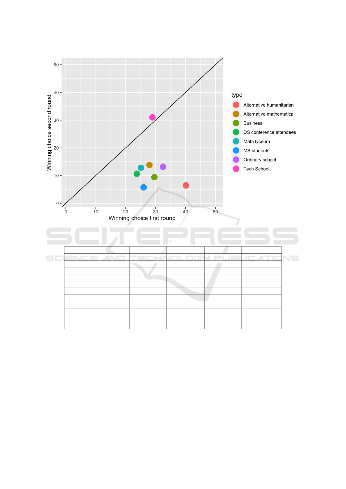
Figure 4: Change in winning number for rounds.
Table 2: Summary of change in strategy levels.
Type b-difference m-difference h-difference inf-difference
Alternative humanitarian -72 -8 0 72
Alternative mathematical -24 -6 30 -6
Alternative humanitarian -52 0 17 43
Math lyceum -9 -36 24 34
Math lyceum -10 -24 28 7
Ordinary school -49 12 20 4
DS conference attendees -14 -32 14 27
MS students -12 -50 50 12
Alternative mathematical -17 -34 23 23
DS conference attendees -17 -30 23 35
Business -32 -17 21 28
Can we in some way establish connection between
number of players and winning number (actually with
strategies, players choose during the game)? To clar-
ify our idea see at 5. It is scatter plot of two-
dimensional variable, x-axis is for number of partici-
pants in the game and y-axis is for winning choice per
round. Different color are for different types of group,
where games was played.
Summarise findings about this plot:
• First and second rounds form two separate clus-
ters. This is expected and inform us that play-
ers learned about the equilibrium concept between
rounds and apply it to practice;
• There are two visible groups inside each round –
undergraduates (schoolchildren, masters) and
adults. Inside each group there is mild tendency
that bigger group has bigger winning number.
This is yet too bold to formulate connection be-
tween size of the group and winning number, but
probably the reason is that when size of the group is
bigger, number of “irrational” players increases. It
can be due to some stable percentage of such persons
in any group or other reasons, but it is interesting con-
nection to investigate.
Guessing Games Experiments in Ukraine. Learning towards Equilibrium
163

Figure 5: Change in winning number for rounds.
3.2 Second Game
In second game the key point is to understand that
almost all strategies are dominated. The results are
presented on figure 6 and we can see that average can
be bigger or smaller then 50, and accordingly win-
ning choice will be 1 or 100. It is worth to note, that
popular nature of these experiments and freedom to
participate make the data gathering not easy. For ex-
ample many participants just didn’t take any decision
in second game. Results are summarised in the ta-
ble 3.
We refine players decisions to see how many play-
ers made choices with rationalizability (Bernheim
(Bernheim, 1984)), which are best response for some
strategy profile of other players. In this game there are
only two best responses possible (in pure strategies),
literally 1 and 100.
This is remarkable result, players without prior
communications choose to almost perfect mixed equi-
librium: almost the same percentage choose 1 and
100. This is even more striking taking into account
no prior knowledge about mixed strategies and mixed
equilibrium, kids play it intuitively and without any
communication. To illustrate the mixed Nash learn-
ing by groups, put dependency of percent of 1 choices
and 100 choices on plot (figure 7).
3.3 Third Game
Third game is simpler then first two, it is coordina-
tion game where players should coordinate without
a word. And, as predicted by Schelling (Schelling,
1980), they usually do. Date presented on figure 8
shows that 1 is natural coordination point, with one
exception – Tech school (id = 1 here) decided that it
would be funny to choose number 69 (it was made
without single word). Probably, it is the age (11th
grade) here to blame. Also we can note attempt to
coordinate around 7, 50 and 100.
Interesting and paradoxical result, which is ex-
pected from general theory, that with fewer options
coordination in fact is more difficult. Lets consider
(figure 9), where players decision was to choose inte-
ger from [1,10], only 10 choices. Comparing to pre-
vious game with 100 possible choices, coordination
was very tricky – two numbers got almost the same
result.
AET 2020 - Symposium on Advances in Educational Technology
164

Figure 6: Statistics for choices.
Table 3: Second game. Rationalizable choices summary.
Type Average Choose 100 Choose 1 Count
Adults 46.5 24.3% 24.34% 115
Alternative mathematical 43.8 25.9% 27.9% 27
Business 50.6 29.3% 29.3% 99
DS conference attendees 37.4 15.8% 36.8% 114
Math lyceum 48.5 22.7% 24.7% 154
Ordinary school 51.2 30.4% 30.4% 23
3.4 Fourth Game
Here we just note, that the winning numbers were:
12, 2, 4, 20. Since no equilibrium here was theoreti-
cally found, we can only gather data at this stage and
formulate hypothesis to found one.
All experimental data and R file for graphs can be
accessed in open repository (Ignatenko, 2021).
4 CONCLUSIONS
In this paper we have presented approach to make ex-
perimental game theory work for learning in educa-
tional process and be a research tool at the same time.
Our result show classical pattern in decision making –
actually every group behave in almost the same way
dealing with unknown game. Some tried to deviate
for unusual actions (like choosing 100 or choosing
69), and this is interesting point of difference with
more “laboratory” setup of existing research. The
main findings of the paper are following:
1. To learn the rules you need to break them. Partic-
ipants have chosen obviously not winning moves
(> 66) partly because of new situation and trou-
ble with understanding the rules. But high percent
of such choices was present in second round also,
when players knew exactly what is going on. This
effect was especially notable in the cases of high
school and adults and almost zero in case of spe-
cial math schools and kids below 9th grade. We
can formulate hypothesis that high school is the
Guessing Games Experiments in Ukraine. Learning towards Equilibrium
165
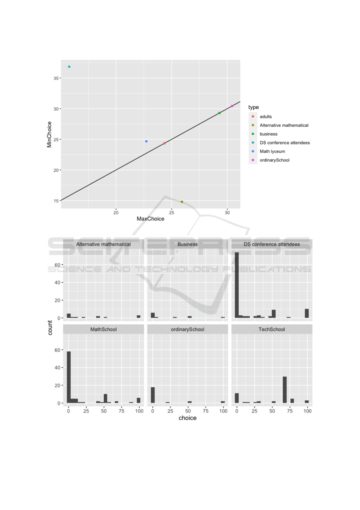
Figure 7: Difference in percent of rationalizable choices.
Figure 8: Histogram of choices.
AET 2020 - Symposium on Advances in Educational Technology
166

Figure 9: Histogram of choices for 1-10 game.
age of experimentation when children discover
new things and do not afraid to do so.
2. If we considered winning number as decision of
a group we can see that group learning fast and
steady. Even if some outliers choose 100, mean
still declines with every round. It seems that
there is unspoken competition between players
that leads to improvement in aggregated decision
even if no prize is on stake. Actually, it is plau-
sible scenario when all participants choose higher
numbers. But this didn’t happen in any experi-
ment. The closest case – Tech school, when bunch
of pupils (posible coordinating) switch to 100 still
only managed to keep mean on the same level.
3. In second game the surprising result is that players
use mixed strategies very well. It is known (from
experiments of Colin Camerer) that chimpanzee
can find mixed equilibrium faster and better than
humans. It seems that concept of mixed strategies
is very intuitive and natural. But still in quite un-
familiar game players made almost equal number
of 1 and 100, so each player unconsciously ran-
domized his own choice.
4. In third game players coordinates to 1, as ex-
pected, because of condition that from numbers
with equal choices – lesser wins. Also we can
note attempts of coordination around 7, 50 and
100. What is interesting is that in practice the
condition was never applied – majority chooses
1 and that’s it. If we decrease the numbers range
to 1-10, other numbers has chance to win (5 or
7 for example). So this is unexpected result –
increasing of number of choices leads to bigger
uncertainty when players trying to find slightest
hint what to do, and this is condition of “lesser
wins”. When players apply this condition to big
area, they probably think – “1 is perfect choice,
and other will think in that way also, this increase
chances of winning”.
The results have multiple applications:
• to provide kids with first hand experience about
strategic interactions and explain their decisions;
• to demonstrate how game theory experiments can
be used in educational process;
• to understand difference in decision making
among groups;
• to compare results with classical experiments and
replicate them in current Ukrainian education sys-
tem.
REFERENCES
Aumann, R. J. (1985). What is game theory trying to ac-
complish? In Arrow, K. and Honkapohja, S., editors,
Frontiers of Economics, pages 5–46. Basil Blackwell,
Oxford. http://www.ma.huji.ac.il/ raumann/pdf/what
Bernheim, B. D. (1984). Rationalizable strate-
gic behavior. Econometrica, 52(4):1007–1028.
http://www.jstor.org/stable/1911196.
Camerer, C. F. (2011). Behavioral game theory: Exper-
iments in strategic interaction. Princeton University
Press.
Crawford, V. P., Costa-Gomes, M. A., and Iriberri, N.
(2013). Structural models of nonequilibrium strategic
thinking: Theory, evidence, and applications. Journal
of Economic Literature, 51(1):5–62.
Fe, E., Gill, D., and Prowse, V. L. (2019). Cognitive skills,
strategic sophistication, and life outcomes. Work-
ing Paper Series 448, The University of Warwick.
https://warwick.ac.uk/fac/soc/economics/research/
centres/cage/manage/publications/448-2019 gill.pdf.
Gill, D. and Prowse, V. (2016). Cognitive ability, charac-
ter skills, and learning to play equilibrium: A level-k
analysis. Journal of Political Economy, 124(6):1619–
1676.
Guessing Games Experiments in Ukraine. Learning towards Equilibrium
167

G
¨
uth, W., Kocher, M., and Sutter, M. (2002). Experimen-
tal ‘beauty contests’ with homogeneous and heteroge-
neous players and with interior and boundary equilib-
ria. Economics Letters, 74(2):219–228.
Ho, T.-H., Camerer, C., and Weigelt, K. (1998). Iterated
dominance and iterated best response in experimental
”p-beauty contests”. The American Economic Review,
88(4):947–969. http://www.jstor.org/stable/117013.
Ignatenko, O. P. (2021). Data from experiments. https://
github.com/ignatenko/GameTheoryExperimentData.
Keynes, J. M. (1936). The General Theory of
Employment, Interest and Money. Palgrave
Macmillan. https://www.files.ethz.ch/isn/125515/
1366 KeynesTheoryofEmployment.pdf.
Mauersberger, F. and Nagel, R. (2018). Chapter 10 - lev-
els of reasoning in keynesian beauty contests: A gen-
erative framework. In Hommes, C. and LeBaron,
B., editors, Handbook of Computational Economics,
volume 4 of Handbook of Computational Economics,
pages 541–634. Elsevier.
Mitzkewitz, M. and Nagel, R. (1993). Experimental results
on ultimatum games with incomplete information. In-
ternational Journal of Game Theory, 22(2):171–198.
Moulin, H. (1986). Game theory for the social sciences.
New York Univeristy Press, New York, 2nd edition.
Nagel, R. (1995). Unraveling in guessing games: An ex-
perimental study. The American Economic Review,
85(5):1313–1326. https://www.cs.princeton.edu/
courses/archive/spr09/cos444/papers/nagel95.pdf.
Schelling, T. (1960). The Strategy of Conflict. Harvard Uni-
versity Press, Cambridge.
Schelling, T. C. (1980). The Strategy of Conflict: With a
New Preface by The Author. Harvard University Press.
AET 2020 - Symposium on Advances in Educational Technology
168
