
Using Dynamic Vector Diagrams to Study Mechanical Motion Models at
Agrarian University with GeoGebra
Leonid O. Flehantov
1 a
, Yuliia I. Ovsiienko
1 b
, Anatolii V. Antonets
1 c
and Vladimir N. Soloviev
2 d
1
Poltava State Agrarian Academy, 1/3 Skovorody Str., Poltava, 36000, Ukraine
2
Kryvyi Rih State Pedagogical University, 54 Gagarin Ave., Kryvyi Rih, 50086, Ukraine
Keywords:
ICT in Learning and Instruction, Teaching the Basics of Mathematical Modeling, Learning of Mechanical
Motion, Visualization Technique in Learning and Instruction, Dynamic Vector Diagrams, GeoGebra.
Abstract:
This article is devoted to study of effectiveness of one of the visualization options we use when teaching
the students of an agricultural university the basics of math modeling. The main goal of this research is to
test the hypothesis that visibility and visualization improve the educational achievements of students if for
visualization we use the dynamic vector diagrams of characteristics of mechanical movement (in particular,
these are velocity and acceleration or the acting force). There are discussion of the methodology and examples
of the use of dynamic vector diagrams when teaching the basics of mathematical modeling. We described how
our students are computing and plotting graphs and dynamic vector diagrams when they doing their practical
learning exercises in math modeling and how they using them to analyze the mechanical motion of a body.
Primarily we research and discuss the effectiveness of using dynamic vector diagrams. Other visualization
options such as using plots of the dynamic characteristics of mechanical movement by Excel and GeoGebra
was discussed earlier in (Flehantov and Ovsiienko, 2019). In this article we described our experience of using
of dynamic vector diagrams in teaching the basics of math modeling at agrarian university and compared the
research results were obtained with previous ones. Also we compare the educational achievements of students
in the basics of math modeling were obtained by them using Excel and by GeoGebra software which allow to
plot and study the dynamic vector diagrams much easy.
1 INTRODUCTION
Recently there are a lot of changes in education tech-
nologies: in fact we are living at a new time. Now it is
clear that some of researches in the field of education
that were made earlier are obsolete. The one of the
main things today is the transition from verbal chan-
nel of communication in learning to visual. Although
the scientists have not yet had time fully to study and
investigate this process but the young people already
have mastered all these.
The approach to teaching the basics of mathemat-
ical modeling (BMM) that this study focuses on is
based on visualization (Ivanova et al., 2020) and it can
be described by the saying: “I hear and forget. I see
a
https://orcid.org/0000-0002-4689-1457
b
https://orcid.org/0000-0002-4873-9061
c
https://orcid.org/0000-0002-2332-6711
d
https://orcid.org/0000-0002-4945-202X
and remember. I do and understand” (Xunzi, 2020).
This article devoted to results of our research on
the impact of visualization to teaching BMM with
the use of popular mathematical computer program –
the GeoGebra dynamic geometry system (GeoGebra,
2021; Kramarenko et al., 2020a). At first, we points
out some researches that were the starting point for
the hypothesis and objectives of this work.
The methodological principles of using ICT in the
teaching of mathematical disciplines at universities
we used were elaborated in (Bobyliev and Vihrova,
2021; Klochko and Bondarenko, 2013; Kramarenko
et al., 2020b; Rakov, 2005; Tarasenkova et al., 2019;
Tryus, 2005). Some important issues of the use of
ICT in the educational process at the universities were
shown in (Abdula et al., 2020; Bakum and Morozova,
2015; Polhun et al., 2021; Spivakovsky et al., 2019;
Hrybiuk et al., 2014).
Note in passing that to using of Excel spreadsheets
in the teaching of BMM which is also mentioned in
336
Flehantov, L., Ovsiienko, Y., Antonets, A. and Soloviev, V.
Using Dynamic Vector Diagrams to Study Mechanical Motion Models at Agrarian University with GeoGebra.
DOI: 10.5220/0010924200003364
In Proceedings of the 1st Symposium on Advances in Educational Technology (AET 2020) - Volume 1, pages 336-353
ISBN: 978-989-758-558-6
Copyright
c
2022 by SCITEPRESS – Science and Technology Publications, Lda. All rights reserved

this article were devoted to a number of scientific pub-
lications about an array of the some aspects of this
direction. For review of the early studies may be of
utility the works by Illia O. Teplytskyi (Teplytskyi and
Semerikov, 2002; Teplytskyi, 2010; Semerikov et al.,
2018).
We can’t be said the same about the GeoGebra dy-
namic geometry system. There are many articles de-
voted to this software but most of them describe of
only the capabilities and show some examples how
to use it in teaching. As examples we can point out
for publication by Osypova and Tatochenko (Osy-
pova and Tatochenko, 2021) on improving the learn-
ing environment for future mathematics teachers with
the use application of the dynamic mathematics sys-
tem GeoGebra AR. In the article by Drushlyak et al.
(Drushlyak et al., 2020) the methodology of forma-
tion of modeling skills based on a constructive ap-
proach was shown the on the example of GeoGebra.
It shows the basic techniques for using GeoGebra in
teaching and studying mathematics, with an empha-
sis on examples from geometry. Noteworthy alone is
the article by Kyslova et al. (Kyslova et al., 2014) de-
voted to the problems of teaching higher mathematics
for students of engineering specialties and to the cre-
ation of dynamic models in GeoGebra.
Caligaris et al. (Caligaris et al., 2015a,b) were
concluded that using GeoGebra applets is an effective
teaching methodology for teaching Calculus. Arbain
and Shukor (Arbain and Shukor, 2015) noted that the
students have more positive perception towards learn-
ing and have better learning achievement using Ge-
oGebra. The article by Vald
´
es y Medina and Medina
Vald
´
es (Vald
´
es y Medina and Medina Vald
´
es, 2015)
is show in practice how the GeoGebra software can
be used to exemplify the different mathematical con-
cepts.
In addition let’s we say that a lot of examples the
using of GeoGebra software for teaching mathematics
and science daily replenished on the GeoGebra web-
site (GeoGebra, 2021; Hall and Lingefjard, 2016). It
is also known that MS Excel has built-in functions for
visualizing changes in calculated values just like Ge-
oGebra has the built-in SpreadSheet component that
allows you to partially perform the tasks the same of
Excel. However, the using of these tools needs the re-
sults of the previous teaching of information technol-
ogy which are not provided for curriculum of agrarian
universities.
The problems of teaching the basics of mathemat-
ical modeling are closely related to the issues of ap-
plied orientation of mathematical (fundamental, natu-
ral sciences) disciplines. In this regard we note the re-
searches (Blomhøj and Kjeldsen, 2006; Blomhøj and
Jensen, 2007; Burghes, 1980; Finlay and King, 1986;
Flores et al., 2016; Geiger et al., 2010; Kaiser et al.,
2011; Kapur, 1982; Klymchuk et al., 2008; Lofgren,
2016; Oke, 1980; Schukajlow et al., 2018; Soloviev
et al., 2019; Temur, 2012; Verschaffel and De Corte,
1997; Vos, 2011). There are some applied issues of
mathematical modeling in agroengineering are con-
sidered in the textbook (Flehantov, 2006).
In general, despite a significant number of stud-
ies and publications, the problems of teaching the ba-
sics of mathematical modeling using ICTs still remain
outside the attention of the integrated approach of re-
searchers.
Our interest for the main topic of this research
based on its practical importance for the train-
ing of modern agricultural production engineers,
since “teaching the basics of mathematical modeling
(BMM) is an important component in the training of
modern agricultural production engineers. Its prac-
tical value is due to the fact that training on the basis
of mathematical modeling can be an effective strategy
in modern realities” (Flehantov and Ovsiienko, 2019).
This research is a logical extension of article (Flehan-
tov and Ovsiienko, 2019) where we also were tested
the hypothesis that visualization of the dynamic char-
acteristics of mechanical processes using GeoGebra
improves the student’s learning outcomes for BMM
(in this article for visualize the dynamic characteris-
tics of mechanical motion were used graphs of trajec-
tories of moved bodies in Excel and GeoGebra).
After the experiment with the simultaneous use of
Excel and GeoGebra we were conducted in the fall of
2018 we observed a reversal of negative dynamics in
the results of training of BMM the students of engi-
neering and technical specialties of the Poltava State
Agrarian Academy, Poltava, Ukraine (PSAA) (2014 –
75.8; 2015 – 75.6; 2016 – 72.6; 2017 – 70.1). Ac-
cording to the results of the fall semester of 2018 the
average score in this discipline was 74.8 (Flehantov
and Ovsiienko, 2019). At the same time in the ex-
perimental groups E (Excel users) and G (GeoGebra
users) we obtained almost the same average values of
student performance, equal to 73.4 and 73.7, in fact at
the level of 2016 (taking into account the permissible
statistical error). Whereas in the EG group (simul-
taneous use of Excel and GeoGebra) the mean value
was 77.4. You can try to explain this result by the fact
that already in 2017 we recognized the negative trend
of lowering student performance as a problem and
showed some enthusiasm in solving it. The results
of the EG group obtained on the basis of the assump-
tion of the leading role of visualization in teaching the
basics of mathematical modeling with the simultane-
ous use of Excel and GeoGebra showed a statistically
Using Dynamic Vector Diagrams to Study Mechanical Motion Models at Agrarian University with GeoGebra
337

significant difference from the results of the E and
G. The average score in the EG group exceeded even
quite high learning outcomes of 2014 and 2015. Thus
it can be already considered now as a fact that the vi-
sualization of modeling results creates additional con-
ditions for improving students’ knowledge taking into
account the specifics of their professional training.
The main goal of this article is to test with new
idea the hypothesis that visibility and visualization
improve the educational achievements of students of
an agricultural university when studying the basics of
mathematical modeling. This research is devoted to
the study of the effectiveness of one of the visual-
ization options, which we use when teaching the ba-
sics of mathematical modeling to students of an agri-
cultural university. As a way of visualization in this
research were used the dynamic vector diagrams of
the characteristics of mechanical movement. Our stu-
dents build these diagrams when they perform practi-
cal educational tasks in mathematical modeling, and
use them to analyze the mechanical motion of a body
thrown at an angle to the horizon, as shown in this ar-
ticle. Further in this article we describe the experience
of using dynamic vector diagrams in teaching the ba-
sics of mathematical modeling, compare the obtained
research results with previous ones and also compare
the educational achievements of students in the ba-
sics of mathematical modeling which were obtained
by them using Excel and GeoGebra.
2 EXPERIMENT DESCRIPTION
2.1 General Design
This article based on the results of the peda-
gogical experiment that was performed by authors
in September-November 2019 and in September-
November 2020. The experiment was enrolled by
167 students of the Faculty of Engineering and Tech-
nology. The provided sample size makes it possible
with ANOVA method to establish significant differ-
ences between group means at the level of 1 point: at
a significance level of 0.05, number of groups 3 and a
power of 80% the required sample size for groups is
at least 50 units.
At the beginning of the experiment the students
was attended were categorized into three groups
called E, G and EG; for this we used the technique
described in (Flehantov and Volchkova, 2010) which
allow us to initially form groups homogeneous by
the criterion of academic performance (Flehantov and
Volchkova, 2012). The group E used Excel spread-
sheets during the training of BMM. The group G used
the GeoGebra. The group EG used simultaneously
Excel and GeoGebra. Throughout the entire study
period, these groups were not permanent: students re-
maining in their academic group could arbitrarily mi-
grate from one experimental group to another. The
final composition of the groups was fixed at the end
of the experiment. All groups underwent BMM train-
ing in a single program using the methodology of a
differentiated approach to training presented in (Fle-
hantov and Ovsiienko, 2019). The training time in all
groups was the same. Each of group was offered com-
plete the same learning task has a direct connection
with the topics important in the training of engineers
of agrarian production. Learning outcomes of the stu-
dents of groups E, G and EG were evaluated on the
results of solving a set of typical tasks for individual
independent work.
The main learning task for all students was: mod-
eling the movement of spherical body was thrown at
an angle to the horizon, with taking into account air
resistance, gravitational interaction, electrostatic in-
teraction, magnetic interaction, etc.
We have applied a differentiated approach in
learning by doing considered the gradual construction
of end-to-end mathematical models (MM) of several
levels of complexity their computer implementation
and study through numerical calculus. The purpose of
these works is to familiarize students with the practice
of creating MM, the construction of computational
circuits and their computer implementation, forming
the skills of conducting a computer experiment and
interpreting its results.
The typical task for the students’ practice was:
create MM of free motion of the body in the grav-
ity field and find its solution. Further we build a cal-
culation algorithm and in the environment of the se-
lected software implement the calculation and com-
puting scheme for MM, conduct a computing exper-
iment and draw conclusions from it. The basic of
such MM is the classical model of the motion of a
body thrown at an angle to the horizon well known
from the school physics course. It’s generalized in the
first year of engineering faculties of agricultural uni-
versities in the study of the discipline “Physics”, also
used in “Higher Mathematics” to illustrate the physi-
cal meaning of the solutions of differential equations
and in the second year in “Theoretical Mechanics”.
Several previously published articles have considered
some options for solving this training exercise using
Excel (Teplytskyi, 2010; Horda and Flehantov, 2015)
and MathCAD (Flehantov and Antonets, 2017). A
similar technique was also used by authors for im-
plementation a differentiated approach in teaching of
BMM (Flehantov and Ovsiienko, 2016). The algo-
AET 2020 - Symposium on Advances in Educational Technology
338

rithm for solving this learning problem has several
stages are described in detail in the article (Flehantov
and Ovsiienko, 2019).
The students’ final learning outcomes were eval-
uated after completing the full course of discipline.
We also retained the methodology for assessing stu-
dent academic achievements: the learning outcomes
of students were assessed on a 100-point scale (Fle-
hantov and Ovsiienko, 2019) on the basis of the per-
formance results of an individual independent learn-
ing problems.
2.2 Mathematical Model Creation
It’s assumed that the students should use the compe-
tencies they acquired were learning “Higher Math-
ematics”, “Physics”, “Theoretical Mechanics”, “Ap-
plied Mathematics”, etc when constructing and ana-
lyzing math models.
The algorithm of actions by students when they
performing the learning exercises is detailed in (Fle-
hantov and Ovsiienko, 2019). The students creates
three mathematical models (MM) in different levels
of complexity named MM I, MM II and MM III using
the mechanical meaning of the derivative and analyz-
ing the vector equations of the resultant forces acting
on the body in three different cases. The MM I model
describes the motion of a body thrown at an angle to
the horizon without air resistance. The MM II model
describes the motion of a spherical body thrown at an
angle to the horizon with air resistance but no rota-
tion. The MM III model additionally takes into ac-
count the Magnus effect – the Magnus force arising
from the rotation of the body during the translational-
rotational motion of the body in dense medium. An
approximate line of reasoning follows next.
Based on the mechanical meaning of the deriva-
tive all models will include these two ordinary differ-
ential equations of the first order:
dx
dt
= v
x
,
dy
dt
= v
y
. (1)
If a body thrown at an angle to the horizon is
affected only by gravity force F
T
=
F
x
1
,F
y
1
then
F
x
1
= 0 and F
y
1
= −mg. Therefore, two more equa-
tions will be added to MM I:
dv
x
dt
= 0,
dv
y
dt
= −g. (2)
The MM I is described by four differential equa-
tions (1) and (2). This elementary model describes
the motion of a body thrown at an angle to the hori-
zon in the field of gravity force without air resistance.
It corresponds to the first (lowest) level of difficulty in
BMM training.
The MM II is the second level of complex-
ity. In this case the equivalent force acting on the
body is F
2
= F
T
+ F
r
, where F
r
= −k
2
v
2
v
v
– force
of air resistance, v =
q
v
2
x
+ v
2
y
– velocity of the
body, k
2
– factor of medium resistance. From here:
F
x
2
= −k
2
v
x
v, F
y
2
= −g − k
2
v
y
v. Thus in addition to
(1) MM II will also include the following two equa-
tions:
dv
x
dt
= −
k
2
m
v
x
q
v
2
x
+ v
2
y
,
dv
y
dt
= −g −
k
2
m
v
y
q
v
2
x
+ v
2
y
.
(3)
MM III corresponds to the third (highest) level
of complexity in our training program. In this case
there will be an equivalent force F
3
= F
T
+ F
r
+ F
M
,
where F
M
= −k
3
v
2
(ω × v), k
3
– coefficient related to
the Magnus effect. From here: F
x
3
= −k
2
v
x
v ± k
3
v
y
v,
F
y
3
= −g − k
2
v
y
v ∓ k
3
v
x
v (the upper sign ”+” is on if
body rotate clockwise, the lower sign “–” is on if body
rotate counterclockwise). Therefore in addition to (1)
MM III will include next two equations:
dv
x
dt
=
−
k
2
m
v
x
±
k
3
m
v
y
q
v
2
x
+ v
2
y
,
dv
y
dt
= −g +
−
k
2
m
v
y
∓
k
3
m
v
x
q
v
2
x
+ v
2
y
.
(4)
In mathematical models we built the following no-
tation used:
x = x(t), y = y(t) – coordinates of center of the
body at the point of time t, s;
v
x
= v
x
(t), v
y
= v
y
(t) – the body’s velocity projec-
tions on axis of reference at time t, m/s;
g – gravity acceleration, m/s
2
; m – mass of the
body (m 6= 0), kg;
k
2
=
1
2
C
D
ρS – factor of medium resistance, kg/m;
k
3
=
1
2
C
L
ρS – factor of Magnus force, kg/m;
C
D
– drag coefficient, depends on body shape and
characteristics of medium (for sphere in air C
D
=
0.47), no the unit of measurement;
C
L
– coefficient characterizing the Magnus effect
depends on the shape of the body, the quality of
its surface and the properties of medium (for sphere
0.1 ≤ C
L
≤ 0.6), no the unit of measurement;
ρ – ambient density (for air = 1, 213), kg/m
3
;
S – normal cross-sectional area of the body rela-
tive to direction of motion, m
2
; in general S = S(t),
for a spherical body S = πr
2
, where r – radius of the
sphere, m.
Using Dynamic Vector Diagrams to Study Mechanical Motion Models at Agrarian University with GeoGebra
339
2.3 Performing the Learning Exercises
by Excel (Group E)
This part of our research we presented here in a con-
cise statement. A detailed description of the relevant
methodology and other explanations are presented in
the article (Flehantov and Ovsiienko, 2016).
The calculation scheme of the computer imple-
mentation of MM I (1), (2) in the MS Excel envi-
ronment is obtained directly from its analytical so-
lution (Klochko and Bondarenko, 2013; Kalitkin and
Koryakin, 2013):
v
xi
= v
0x
,v
yi
= v
0y
− gt
i
,x
i
= x
0
+ v
0x
t
i
,
y
i
= y
0
+ v
0y
t
i
−
gt
2
i
2
,i = 0, n
(5)
The following notation used here:
x
0
, y
0
– initial coordinates the center of the body,
m;
v
0
– initial velocity of the body, m/s;
α
0
– initial angle to the horizon which the body is
thrown, radians;
v
0x
= v
0
cosα
0
, v
0y
= v
0
sinα
0
– projections the
initial velocity of the body v
0
;
t
i
= i · ∆t,t
i
∈ [0, t
M
],i = 0, n – the time points of
observation; i – numbers of body observation posi-
tions (fixation points); n – numbers of fixation points;
∆t = t
M
/n – time between the time points of observa-
tion, s; t
M
– simulation time, s;
x
i
= x(t
i
), y
i
= y(t
i
) – coordinates the center of the
body in the time point t
i
;
v
xi
= v
x
(t
i
), v
yi
= v
y
(t
i
) – projections velocity of
the body in the time point t
i
; v
i
=
q
v
2
xi
+ v
2
yi
– veloc-
ity of the body in the time point t
i
.
Models MM II (1), (3) and MM III (1), (4), unlike
MM I, do not allow an analytical solution. Therefore
the computational schemes of the models are based
on numerical methods.
The computational scheme for MM II according
to the Euler method for the fist order ODE systems is
(Kalitkin and Koryakin, 2013):
v
x i+1
= v
xi
−
k
2
m
v
xi
v
i
∆t,
v
y i+1
= v
yi
−
g +
k
2
m
v
yi
v
i
∆t,
x
i+1
= x
i
+ v
xi
∆t,y
i+1
= y
i
+ v
yi
∆t.
(6)
For MM III the calculation scheme is the same but
the first two equations in (6) need to replace by fol-
lowing ones:
v
x i+1
= v
xi
−
k
2
m
v
xi
v
i
− rot
k
3
m
v
yi
v
i
∆t,
v
y i+1
= v
yi
−
g +
k
2
m
v
yi
v
i
+ rot
k
3
m
v
xi
v
i
∆t.
(7)
The initial data for calculations by formulas (5),
(6), (7) are the values of parameters g, x
0
, y
0
, v
0
, α
0
,
r, m, ρ , C
D
, C
L
, t
0
, t
M
, n and rot. The rot param-
eter can take three fixed values: (–1) – means coun-
terclockwise rotation, (+1) – clockwise rotation, 0 –
no rotation. Model MM III with rot = −1 further we
denote as MM III–, and with rot = +1 – as MM III+.
With rot = 0 the model MM III is equally matched to
model MM II.
Numerical calculations by formulas (5), (6), (7)
are performed by standard MS Excel tools. As a result
the next tables of values are obtained: i, t
i
, x
i
, y
i
, v
xi
,
v
yi
, v
i
, α
i
, E
ki
, E
pi
, where α
i
= arctg
v
yi
v
xi
– the angle of
the trajectory of the body to the horizon; E
ki
=
mv
2
i
2
–
kinetic energy of translational motion of the body;
E
pi
= mgy
i
– the potential energy of the body.
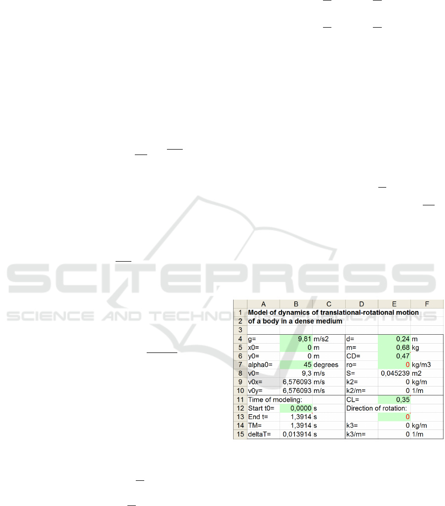
Figure 1 demonstrates of the data input interface
of the models MM I, MM II and MM III in MS Ex-
cel. Figure 2 displays a part of table of calculations
according to MM III for values of input parameters
presented in figure 1.
Figure 1: Interface for input of initial data for math models
MM I – MM III in MS Excel.
Figure 3 and figure 4 depicts the plots of trajec-
tories and velocities of the bodies calculated for all
the models under consideration. Visual comparison
and analysis of such graphs allows students to formu-
late meaningful conclusions about the characteristics
of those movements in various conditions.
In this way, the students using Excel analyze the
obtained numerical results and graphs by changing
the input parameters of the models. Thus, they can
to study the motion of body thrown at an angle to the
AET 2020 - Symposium on Advances in Educational Technology
340
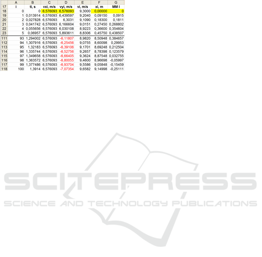
Figure 2: Fragment of the table of calculations for MM I in
MS Excel.
horizon in various conditions to answer by itself to
control questions and to prepare to exam.
2.4 Performing the Learning Exercises
by GeoGebra (Group G)
The description and implementation of the mathe-
matical model of the mechanical motion of bodies
in GeoGebra has its own characteristics, which we
were mentioned in the work (Flehantov and Ovsi-
ienko, 2019).
The main feature of GeoGebra is an algebraic-
geometric approach to the description of mathemat-
ical objects. To solve MM I, MM II and MM III by
GeoGebra is much easier than by Excel. In GeoGe-
bra is not necessary to build and describe in detail
(step by step) complex calculation schemes for solv-
ing systems of differential equations of models. All
you need is write down the models following the Ge-
oGebra syntax and use the built-in NSolveODE com-
mand for numerical solutions of first order differential
equations (wiki.geogebra.org, 2020).
The MM I represents in GeoGebra by formulas (1)
and (2) as follow (all commands are entered through
the command line of the program). From now on the
GeoGebra’s notation used:
x1’(t,x1,y1,vx1,vy1) = vx1
y1’(t,x1,y1,vx1,vy1) = vy1
vx1’(t,x1,y1,vx1,vy1) = 0
vy1’(t,x1,y1,vx1,vy1) = -g
Next input command used to solve the system of
differential equations above by GeoGebra is:
NSolveODE({x1’,y1’,vx1’,vy1’},
0,{x0,y0,vx0,vy0},TM)
The NSolveODE command implements the 4th
order numerical Runge-Kutta method in GeoGebra
command line (GeoGebra, 2021; Hall and Linge-
fjard, 2016; wiki.geogebra.org, 2020). It gener-
ates the numerical solution the Cauchy problem
per segment t ∈ [0, t
M
] with initial conditions
{x0, y0, vx0, vy0} and other input parameters
of model – tabulates four functions x
1
= x
1
(t),
y
1
= y
1
(t), v
x1
= v
x1
(t), v
y1
= v
y1
(t) (according
to the number of unknown functions in the model).
The resulting solutions are assigned with identifiers
called numericalIntegral with sequential number-
ing (according to the order of unknown functions in
the system of differential equations), namely:
numericalIntegral1 = x1(t)
numericalIntegral2 = y1(t)
numericalIntegral3 = vx1(t)
numericalIntegral4 = vy1(t)
The same way, the MM II by formulas (1) and (3)
is represented as:
x2’(t,x2,y2,vx2,vy2)=vx2
y2’(t,x2,y2,vx2,vy2)=vy2
vx2’(t,x2,y2,vx2,vy2)=-k_2*vx2
*sqrt(vx2ˆ2 + vy2ˆ2)/m
vy2’(t,x2,y2,vx2,vy2)=-g - k_2*vy2
*sqrt(vx2ˆ2 + vy2ˆ2)/m
We find the solution of the MM II by the com-
mand:
NSolveODE({x2’,y2’,vx2’,vy2’},0,
{x0,y0,vx0,vy0},TM)}
This command also gives us four functions – MM
II solution:
numericalIntegral5 = x2(t)
numericalIntegral6 = y2(t)
numericalIntegral7 = vx2(t)
numericalIntegral8 = vy2(t)
Same as previous the MM III by formulas (1) and
(4) is represented next way:
x3’(t,x3,y3,vx3,vy3)=vx3
y3’(t,x3,y3,vx3,vy3)=vy3
vx3’(t,x3,y3,vx3,vy3)=-k_2*vx3*
sqrt(vx3ˆ2+vy3ˆ2)/m+rot*k_3*vy3*
sqrt(vx3ˆ2+vy3ˆ2)/m
vy3’(t,x3,y3,vx3,vy3)=-g-k_2*vy3*
sqrt(vx3ˆ2+vy3ˆ2)/m-rot*k_3*vx3*
sqrt(vx3ˆ2+vy3ˆ2)/m
And the MM III solution we will find by the com-
mand:
NSolveODE({x3’,y3’,vx3’,vy3’},0,
{x0,y0,vx0,vy0},TM)}
This way we have got the MM III solution:
numericalIntegral9 = x3(t)
numericalIntegral10 = y3(t)
numericalIntegral11 = vx3(t)
numericalIntegral12 = vy3(t)
Now then we have saw that due to the unifor-
mity of actions the solutions of all three models are
obtained by GeoGebra much faster than with Excel.
Using Dynamic Vector Diagrams to Study Mechanical Motion Models at Agrarian University with GeoGebra
341
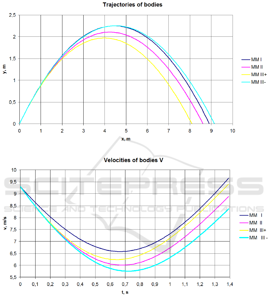
Figure 3: Plots of trajectories of bodies for MM I – MM III in MS Excel.
Figure 4: Graphs of velocities of bodies for MM I – MM III in MS Excel.
Also, if the students have this solutions, than they can
fast and easy visualizing dynamic characteristics of
the math models by GeoGebra as it shown in figure 5.
The trajectories of bodies visualized in GeoGebra
according to the models MM I, MM II and MM III
using the values of functions x1(t), y1(t), x2(t),
y2(t), x3(t), y3(t) as coordinates for three moving
points A=(x1, y1), B=(x2, y2) and C=(x3, y3)
respectively. Figure 5 shows the trajectories of spher-
ical bodies thrown at an angle to the horizon (for three
different values of initial angles) for models: MM I –
red line; MM II – green line; MM III – blue line.
These colors we will use for convenience in all fig-
ures next. The current values of the basic parameters
of the models are shown in the figure on the interac-
tive controls. The arrows shown in figure 5 are vectors
AET 2020 - Symposium on Advances in Educational Technology
342
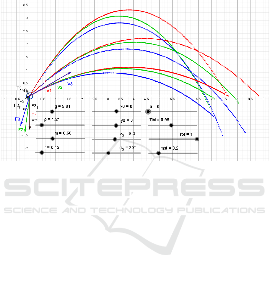
Figure 5: Graphs of trajectories of bodies for MM I – MM III in GeoGebra for different values of initial angles α
0
: 30
◦
, 45
◦
and 60
◦
.
of velocities and vectors of forces acting on the bodies
as they moves.
As we see, the GeoGebra software has better
graphics than Excel and provides additional visual-
ization capabilities. In particular, using the animation
feature, the students can observe with GeoGebra dy-
namic graphing of functions – a computer simulation
the process of mechanical movement of the body. By
using dynamic zooming in the GeoGebra window the
students can to view graph details on a larger scale.
Figure 6 and figure 7 shows some fragments trajecto-
ries of bodies for opposite directions of body rotation
which controlled in MM III by parameter rot. The
plots in these figures are presented for compare one
to others as an example.
Vectors of velocities of the bodies in
figure 6 and figure 7 describes in GeoGe-
bra as follow: V1=Vector(A, A3), where
A3=(x(A1), y(A2)), A1=(x(A)+mst*y(Point(
numericalIntegral3, c)), y(A)) or A1=(x(A)
+ mst*vx1,y(A)), A2=(x(A),y(A)+mst*y(Point
(numericalIntegral4,c))) or A2=(x(A),y(A)
+mst*vy1); V2=Vector(B,B3), where
B3=(x(B1),y(B2)), B1=(x(B)+mst*y(Point
(numericalIntegral7, c)), y(B)) or B1=
(x(B)+mst*vx2,y(B)), B2=(x(B),y(B)+mst
*y(Point(numericalIntegral8,c))) or B2=
(x(B),y(B)+mst*vy2); V3=Vector(C,C3), where
C3=(x(C1),y(C2)), C1=(x(C)+mst*y(Point
(numericalIntegral11, c)), y(C)) or C1=
(x(C)+mst*vx3,y(C)), C2=(x(C),y(C)+mst*y
(Point(numericalIntegral12,c))) or C2=
(x(C),y(C)+mst*vy3);
mst – scale factor for displaying vectors used
for convenience because in normal scale they can
be disproportionate in size – some much larger than
others (in figure 5, figure 6 and figure 7 value of
mst = 0.1).
Vectors of forces acting on the bodies and their
resultants for three different models are represented
in figure 6 and figure 7 (in order of construction).
Indices 1, 2 and 3 are referring to models MM I, MM
II and MM III respectively:
F1=Vector(A,F1_1), where F1 1=(x(A),y(A)
-mst*m*g);
F2=Vector(B,F2_3), where F2_3=F2_1 + F2_2-B,
F2_1=(x(B),y(B)-mst*m*g),
F2_2=(x(B) + mst*F2x_r, y(B) + mst*F2y_r),
F2x_r= -k_2*vx2*sqrt(vx2ˆ2 + vy2ˆ2),
F2y_r= -k_2*vy2*sqrt(vx2ˆ2 + vy2ˆ2);
F2_T= Vector(B,F2_1); F2_r= Vector(B,F2_2);
F3= Vector(C, F3_5), where F3_5=F3_3+F3_4-C,
F3_3= F3_1 + F3_2-C,
F3_4= (x(C) + mst*F3x_M, y(C) + mst*F3y_M),
Using Dynamic Vector Diagrams to Study Mechanical Motion Models at Agrarian University with GeoGebra
343
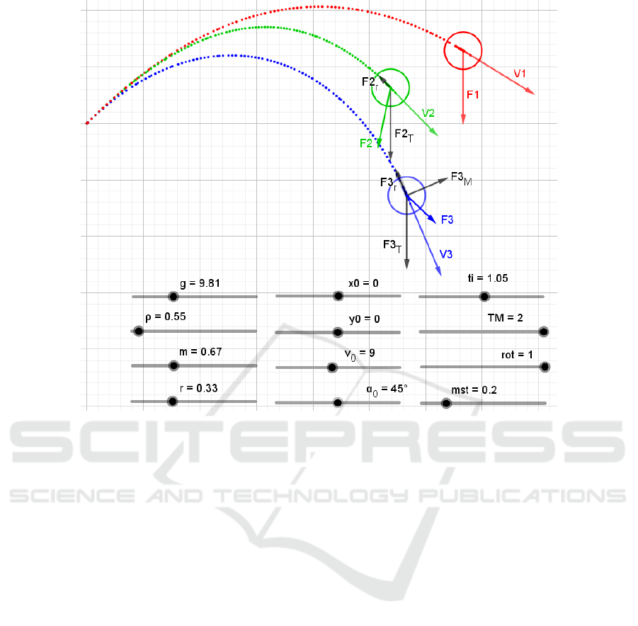
Figure 6: Fragments of trajectories of bodies plotted in GeoGebra for MM I – MM III with rot=+1.
F3_1= (x(C), y(C) - mst*m*g),
F3_2= (x(C) + mst*F3x_r, y(C) + mst*F3y_r),
F3x_r=-k_2*vx3*sqrt(vx3ˆ2 + vy3ˆ2),
F3y_r=-k_2*vy3*sqrt(vx3ˆ2 + vy3ˆ2),
F3x_M=rot*(-k_3)*vy3*sqrt(vx3ˆ2 + vy3ˆ2),
F3y_M=rot*k_3*vx3*sqrt(vx3ˆ2 + vy3ˆ2).
Vectors of the gravity force F3
T
, the force of air
resistance F3
r
and the Magnus force F3
M
for model
M III are represented as follows:
F3_T=Vector(C,F3_1),
F3_r=Vector(C,F3_2),
F3_M=Vector(C,F3_4).
Thus, the students implements the mathematical
models MM I, MM II, MM III in the GeoGebra en-
vironment with the help of this simple mathematical
apparatus based on the method of coordinates and el-
ementary vector algebra.
Figure 8, figure 9 and figure 10 shows the dy-
namic vector diagrams which our students are plot-
ting in GeoGebra and studying by computer simu-
lation. On them in dynamics are displayed the vec-
tor diagrams of the velocities of bodies and their
projections in different phases of motion according
to the models MM I, MM II, MM III. These dia-
grams are dynamic and interactive because they au-
tomatically changes if you use the sliders shown in
the figure to set new values for the model inputs.
At moment represented results at time ti = 1.04 s
for the following values of the initial parameters:
g=9.81, ro=1.213, m=0.68, r=0.12\verb, x0=0,
y0=0, v0=9.3, alpha0=45, rot=1, mst=0.1.
The using of dynamic vector diagrams for visu-
alizing dynamic characteristics to study and analyze
mechanical movement when teaching students the ba-
sics of mathematical modeling is the main difference
between this studies from the previous ones. The
computer simulation and the studying dynamic vec-
tor diagrams of velocities of bodies allows for stu-
dents interactively observe changes that occur with
vectors of velocities depending on changes of values
of various model parameters and study and compare
the dynamic characteristics of motion of the bodies in
different phases of its movement.
The students simultaneously study and analyze the
corresponding plots of velocities of the bodies and
their projections on the coordinate axes similar to
those shown in figure 11 and figure 12. In contrast to
vector diagrams these plots better shows how changes
the absolute value of velocity of the body. The anal-
ysis allow to us to find the direction of movement of
body at different times. At the same time dynamic
vector diagrams of velocities give us a clear visual
AET 2020 - Symposium on Advances in Educational Technology
344
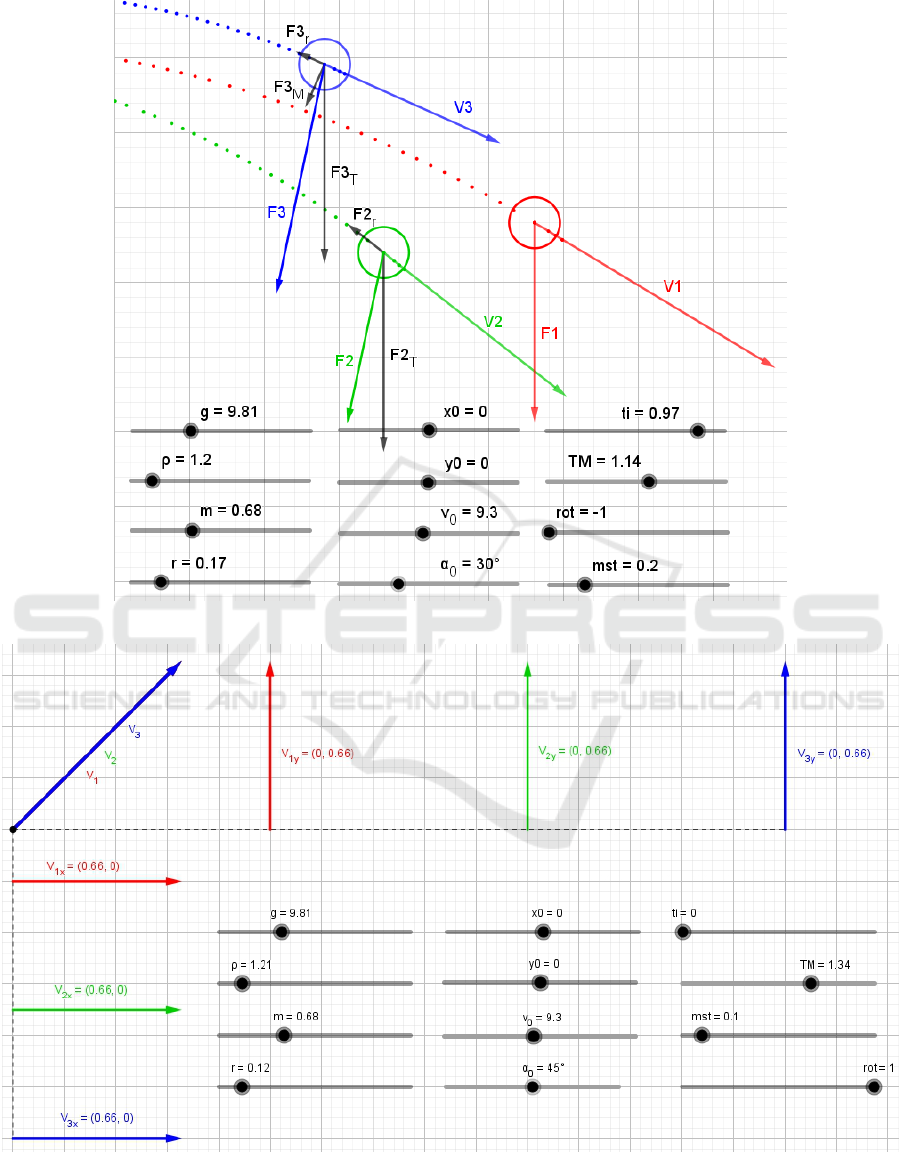
Figure 7: Fragments of trajectories of bodies plotted in GeoGebra for MM I – MM III with rot=-1.
Figure 8: The dynamic vector diagram of velocities of bodies plotted in GeoGebra for MM I – MM III+ (clockwise rotation)
at start of movement: ti=0, rot = +1.
Using Dynamic Vector Diagrams to Study Mechanical Motion Models at Agrarian University with GeoGebra
345
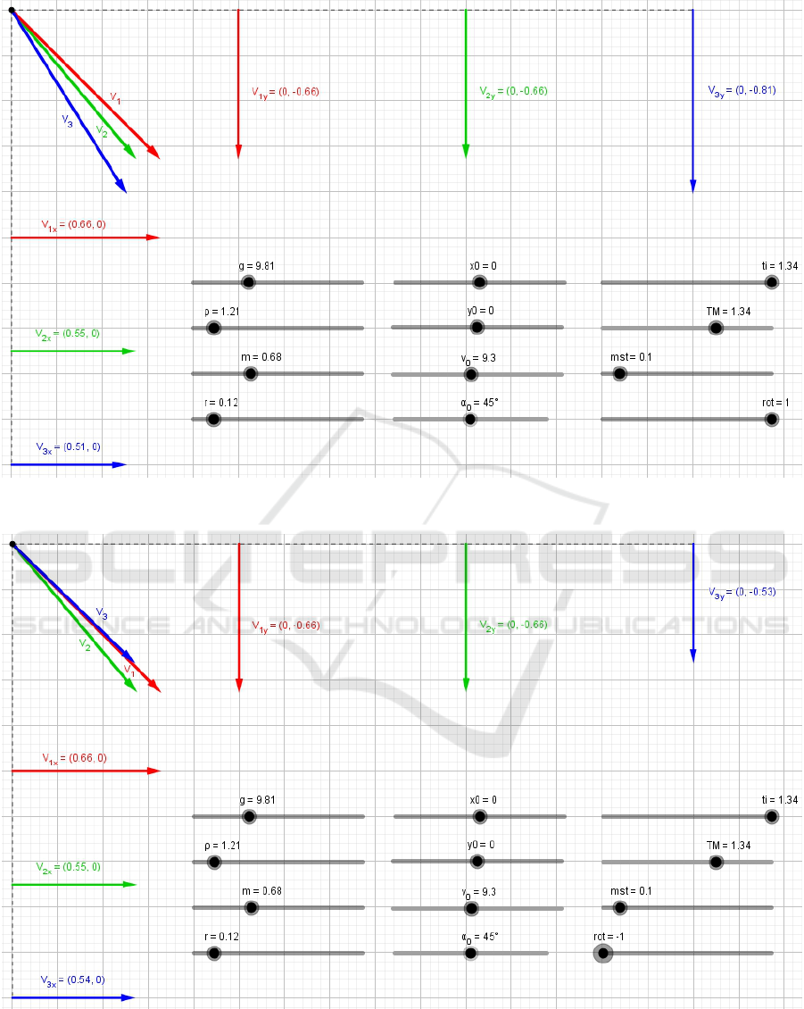
Figure 9: The dynamic vector diagram of velocities of bodies plotted in GeoGebra for MM I – MM III+ (clockwise rotation)
at the end of motion: ti=1.34, rot=+1.
Figure 10: The dynamic vector diagram of velocities of bodies plotted in GeoGebra for MM I – MM III- (counterclockwise
rotation) at the end of motion: ti=1.34, rot=-1.
representation not only of the absolute value of the
body’s velocity and its projections (this can be judged
by the length of the corresponding vectors) but also of
the direction of motion of the body (this can be seen
AET 2020 - Symposium on Advances in Educational Technology
346

directly in the direction of the vector of body veloc-
ity).
Figure 11 allow us to compare the plots of the hor-
izontal projections of velocity of the body vx1(t),
vx2(t), vx3(t) for the three different models MM I,
MM II and MM III for two cases: when rot=+1
(clockwise rotation) and rot=-1 (counterclockwise
rotation). Studying these plots provides for the stu-
dents a lot of useful information about the features of
body movement thrown at an angle to the horizon un-
der different conditions. In particular, these plots are
shows clearly that when rotated clockwise the body at
the beginning of the movement accelerates in the hor-
izontal direction and then slows down. On the con-
trary, for rot=-1 the body slows down at first, but
somewhat accelerates at the end of the movement.
The GeoGebra allows us to build similar plots and
diagrams for all functions that are the solution of the
models. Performing their interactive comparisons at
various values of the parameters of the models we
can quickly conduct a mini-study to establish the all
necessary facts or identify the patterns. For example,
the Fig. 12 shows the plots of the functions y1(t),
y2(t), y3(t) for the MM I, MM II, MM III when
rot=1 and rot=-1. Changing the time of simulation
TM we can quickly set the time point when the body
touches the surface of the earth (determine the flight
time). As you see, for identical input parameters of
the model, the body rotating clockwise will fall to the
surface of the earth in 1.14 s and the body rotating
counterclockwise will be flying 1.46 s. This technique
ensures the effective formation of research competen-
cies of the students.
Similarly, our students study and analyze the
forces acting on the body during movement and their
resultants, as well as their projections. Performing
computer simulations in Excel and GeoGebra based
on the created mathematical models they observe and
analyze, for example, how these vector quantities
change at different points in time, what are the ten-
dencies of these changes, what they mean and what
they indicate. The corresponding illustrations using
GeoGebra will be given below. This approach con-
tributes to formation of the analytical abilities and de-
velopment of skills of graphic analysis of students.
2.5 Performing the Learning Exercises
with Excel and GeoGebra (Group
EG)
The experimental group EG performed the same
learning exercises using simultaneously Excel and
GeoGebra in accordance with methodology described
above.
The participants of this group used Excel (if feel
it necessary or expedient, in particular, for numeri-
cal calculations or for presenting the results in tabular
form) or the GeoGebra software for visual representa-
tion and analysis the dynamic characteristics in form
of plots and dynamic vector diagrams. As example
of these works you may see the vector diagrams of
the forces acting on the body plotting according to
the models M I, MM II and MM III in figure 13 and
figure 14.
3 RESULTS
The table 1 shows the results of final learning out-
comes of students of the Faculty of Engineering and
Technology of the agricultural university at the end of
the experiment described in this article: training the
basics of mathematical modeling using visualization
of the dynamic characteristics of mechanical move-
ment in the form of dynamic vector diagrams. The
final learning outcomes of the students of groups E,
G and EG were evaluated on the results of solving
a set of typical learning problems or individual inde-
pendent works. These results are presented here on a
100-point scale (Flehantov and Ovsiienko, 2019).
The primary statistical data processing results of
the experiment (table 2) are showed that the average
scores in all groups (mean) are different. The means
for groups E and G close to each other (73.36 and
73.85) but both lower than the mean of group EG
(78.25). The mean values in groups E and G almost
coincide with similar indicators in the same groups
of the previous years: MeanE=73.36 (2019) vs. 73.4
(2018); MeanG=73.85 (2019) vs. 73.7 (2018). At
the same time the mean value in group EG-2019
exceed the corresponding figure in group EG-2018:
MeanEG=78.25 (2019) vs. 77.4 (2018). The result of
Shapiro-Wilk test shows the trust of hypothesis about
normal data distribution in all groups.
Analysis of variance (ANOVA) showed a sta-
tistically significant difference in average values of
learning outcomes (Score/Point/Bal) in all groups
(F = 4.678693; p = 0.010613) (table 3). The post-
hoc comparison for means of groups E vs. G, E vs.
EG, G vs. EG shows that the difference between the
means of groups E and G is within the statistical er-
ror (table 4). The pair-wise post-hoc comparisons
results indicate the statistical significance of the dif-
ference between the mean for group EG and the mean
groups E and G.
Using Dynamic Vector Diagrams to Study Mechanical Motion Models at Agrarian University with GeoGebra
347
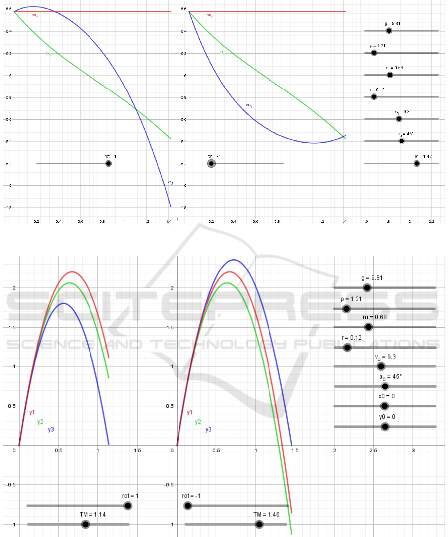
Figure 11: The visual study in GeoGebra: how changes the projection v
x
for math models MM I, MM II, MM III+ (rot = +1,
clockwise rotation) and MM III- (rot=-1, counterclockwise rotation).
Figure 12: The visual study in GeoGebra: how long is the spherical body flight in air according to different math models if
the body rotate clockwise and counterclockwise? (rot=+1 and rot=-1).
4 DISCUSSION
In this article we made compare the earlier results we
obtained when our students at first used Excel spread-
sheets as the tool for solving learning exercises and
then the GeoGebra dynamic geometry system was
added. At the same time during the training sessions
AET 2020 - Symposium on Advances in Educational Technology
348
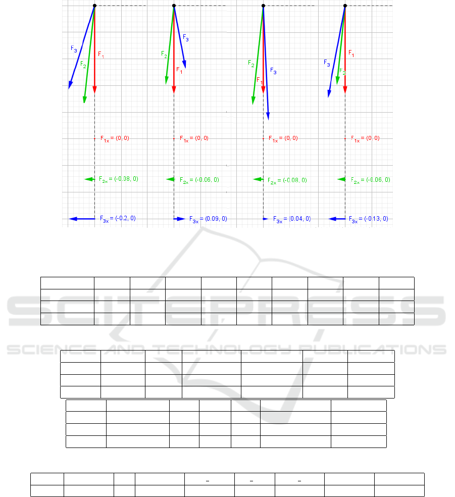
Figure 13: The dynamic vector diagram of X-component F
x
of the resultant of the forces acting on the body in the four cases
of flight: ti = 0, rot = 1; ti = TM, rot = 1; ti = 0, rot = -1; ti = TM, rot = -1.
Table 1: Final learning outcomes of students after the experiment.
Score 50-55 55-60 60-65 65-70 70-75 75-80 80-85 85-90 90-95
Group E 1 2 6 9 14 10 7 4 -
Group G - 3 6 10 13 15 8 3 1
Group EG - 1 3 5 10 15 9 7 5
Table 2: Primary statistical data processing results.
Group Valid N Mean Conf.-95% Conf.+95% Median Mode
E 53 73.36 71.16 75.55 74 Multiple
G 59 73.85 71.74 75.95 74 76
EG 55 78.25 75.94 80.57 77 76
Group Freq. Mode Min Max SD Shapiro-Wilk test
E 5 55 90 7.96 W=0.98823 p=0.87840
G 5 56 91 8.08 W=0.98749 p=0.80486
EG 6 60 95 8.56 W=0.98158 p=0.55809
Table 3: ANOVA results.
SS df MS SS Err df Err MS Err F p
Point 1249.818 2 624.9091 10588.73 164 64.56544 4.678693 0.010613
we consistently and systematically studied how vari-
ous methods and techniques of visualizing the results
of modeling affect the results of educational achieve-
ments of students who study at the agrarian univer-
sity (the specifics of teaching this group of students
to mathematical disciplines were discussed by us ear-
lier).
Based on the above we conclude that visualization
of the dynamic characteristics of mechanical move-
ment in the form of dynamic vector diagrams using
the GeoGebra software allow to improve the educa-
tional achievements of students of the agrarian univer-
sity when studying the basics of mathematical model-
ing.
There are several possible reasons for this result.
At first, since implementation of mathematical mod-
els in MS Excel, in fact, is a stepwise reproduction
of the sequence of the mathematical operations by
means of spreadsheets, than their use contributes to
a better understanding of the students of the technical
Using Dynamic Vector Diagrams to Study Mechanical Motion Models at Agrarian University with GeoGebra
349
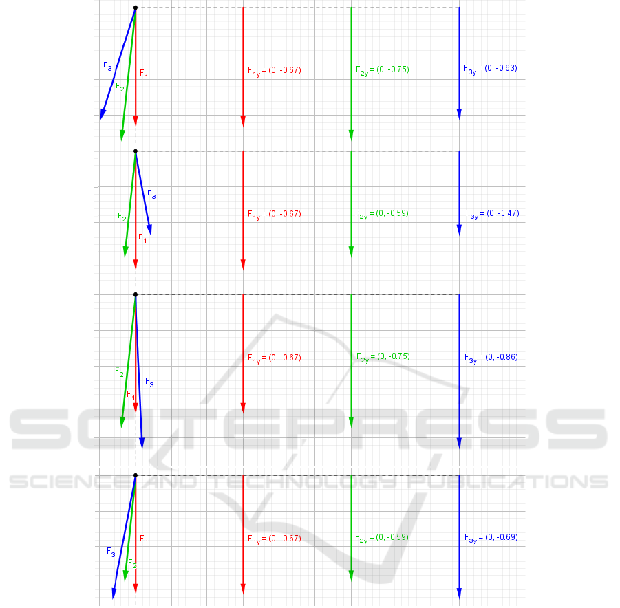
Figure 14: The dynamic vector diagram of Y-component F
y
of the resultant of the forces acting on the body in four cases
(from top to right): ti = 0, rot = 1; ti = TM, rot = 1; ti = 0, rot = -1; ti = TM, rot = -1.
component of mathematical modeling, provides them
with the opportunity to diagnose calculations by it-
self, and also creates additional didactic benefits for
the teacher, such as being able to identify and discuss
with students all the intermediate effects and simu-
lation outcomes that may remain invisible (hidden)
when using professional computer math systems such
as Mathcad (Flehantov and Antonets, 2017), Mathe-
matica, MATLAB or Maple, etc.
In addition, visualization of the trajectory of me-
chanical motion of bodies in the form of Excel charts
provides the formation of intuitive ideas about how
the characteristics of movement of bodies changes de-
pending on the initial conditions and other parame-
ters. This allows to students to acquire the skills of
consciously adjusting input parameters to achieve the
desired simulation result. However the standard Excel
features do not allow them to visualize the changes in
the instantaneous velocities and the direction of mo-
tion of bodies along their trajectories. Therefore us-
ing of Excel in training does not create sufficient con-
ditions for the formation of skills to analyze the dy-
namic characteristics of movement based on numeri-
cal data.
AET 2020 - Symposium on Advances in Educational Technology
350
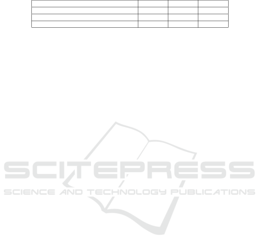
Table 4: Pair-wise post-hoc comparisons results.
Pair-wise post-hoc comparisons of means E vs. G E vs. EG G vs. EG
LSD-test p>0.9468 p<0.0262 p<0.0120
Duncan-test p>0.9475 p<0.0135 p<0.0151
Tukey HSD for unequal N test p>0.9977 p<0.0061 0.0048
On the other hand the GeoGebra allows to the stu-
dents to form their intuitive spatial perceptions faster
by visual analyzing dynamic motion characteristics.
In our view this is made possible primarily by the dy-
namic visualization of vector characteristics of mo-
tion. We observed that after completing the proposed
learning exercises with the help of GeoGebra the stu-
dents more easy formulated the meaningful answers
to questions of qualitative evaluation. Studying the
dynamic plots such as figure 11 in an interactive mode
allows them quickly and accurately answer the ques-
tions such as: “How does the change the direction of
rotation will affect the linear velocity of the body?”,
“At what points in time the velocity of the body will
in airless space be equal to the speed of the body in
air?” and so on. However, the students who were
working in Excel environment were better at answer-
ing questions about the quantitative characteristics of
the models.
That’s why as in our previous study (Flehantov
and Ovsiienko, 2019, 2016) we are of the opinion that
using only GeoGebra to study the basics of modeling
creates the inconvenience to evaluate the simulation
results in a numerical dimension. Therefore it does
not provide a sufficient level of skills to numerically
evaluate the characteristics of the phenomenon or the
simulated process. At the same time the wide using of
GeoGebra during BMM training contributes to the ef-
fectively formation of intuitive spatial representations
that are very important for engineering professionals.
Because, as in the previous study, there is no signif-
icant difference between final learning outcomes in
groups E and G, this could mean that simultaneous
use of Excel and GeoGebra compensates for these
shortcomings and therefore provides the best educa-
tional achievements. At the same time, the using of
dynamic vector diagrams in GeoGebra environment
to learning the basics of mathematical modeling fur-
ther up these results.
5 CONCLUSION
The analysis of the data we collected shows that
the students who simultaneously used GeoGebra and
Excel at the highest level of learning difficulty in
dynamic vector diagram visualization mode demon-
strated a better understanding of mathematical model-
ing problems and improved their ability to use math-
ematical modeling to solve problems. At the same
time, we found no statistically significant difference
in learning outcomes between groups of students who
used only Excel or only GeoGebra separately during
BMM training. In addition, we noticed that students
who used Excel for computer modeling responded
better to quantitative questions of exam. The students
who performed their learning exercises exclusively in
the GeoGebra environment were much better at deal-
ing with quality questions.
Results of this study we get conclusion that the si-
multaneous use of Excel and GeoGebra with vizual-
isation mode by dynamic vector diagrams demon-
strated improved the academic achievement of stu-
dents with BMM. This is indicated by the statisti-
cally significant difference between the average re-
sults of students’ academic achievement, shown in ta-
ble 2 confirmed with the results of table 3 and table
4.
So, this research show that the proper use of ap-
propriate software to visualize the dynamic charac-
teristics of mathematical models in the context of the
teaching BMM at an agrarian university is an effec-
tive way to improve student performance. We were
concluded that the hypothesis that visualization of the
characteristics of mechanical movement by the dy-
namic vector diagrams can to improve the educational
achievements of students is true. However the as-
sumption that visualizing the results of modeling us-
ing GeoGebra in conjunction with a differentiated ap-
proach to learning creates additional conditions for
improving students’ knowledge, taking into account
the specifics of their vocational training requires fur-
ther verification.
REFERENCES
Abdula, A., Baluta, H., Kozachenko, N., and Kassim, D.
(2020). Peculiarities of using of the Moodle test tools
in philosophy teaching. CEUR Workshop Proceed-
ings, 2643:306–320.
Arbain, N. and Shukor, N. A. (2015). The effects of geoge-
bra on students achievement. Procedia - Social and
Behavioral Sciences, 172:208–214.
Bakum, Z. and Morozova, K. (2015). Didactical conditions
Using Dynamic Vector Diagrams to Study Mechanical Motion Models at Agrarian University with GeoGebra
351

of development of informative-communication com-
petence of future engineers during master preparation.
Metallurgical and Mining Industry, 7(2):164–167.
Blomhøj, M. and Jensen, T. (2007). What’s all the fuss
about competencies?: Experiences with using a com-
petence perspective on mathematics education to de-
velop the teaching of mathematical modelling. New
ICMI Study Series, 10:45–56.
Blomhøj, M. and Kjeldsen, T. (2006). Teaching mathe-
matical modelling through project work - experiences
from an in-service course for upper secondary teach-
ers. ZDM - International Journal on Mathematics Ed-
ucation, 38(2):163–177.
Bobyliev, D. Y. and Vihrova, E. V. (2021). Problems and
prospects of distance learning in teaching fundamental
subjects to future mathematics teachers. Journal of
Physics: Conference Series, 1840(1):012002.
Burghes, D. (1980). Mathematical modelling: A positive
direction for the teaching of applications of mathe-
matics at school. Educational Studies in Mathematics,
11(1):113–131.
Caligaris, M., Rodr
´
ıguez, G., and Laugero, L. (2015a).
Learning styles and visualization in numerical anal-
ysis. Procedia - Social and Behavioral Sciences,
174:3696–3701.
Caligaris, M. G., Schivo, M. E., and Romiti, M. R. (2015b).
Calculus & geogebra, an interesting partnership. Pro-
cedia - Social and Behavioral Sciences, 174:1183–
1188.
Drushlyak, M. G., Semenikhina, O. V., Proshkin, V. V.,
Kharchenko, S. Y., and Lukashova, T. D. (2020).
Methodology of formation of modeling skills based
on a constructive approach (on the example of GeoGe-
bra). CEUR Workshop Proceedings, 2879:458–472.
Finlay, P. and King, M. (1986). Teaching management
students to love mathematical modelling. Teaching
Mathematics and its Applications, 5(1):31–37.
Flehantov, L. and Antonets, A. (2017). Computer simu-
lation the mechanical movement body by means of
MathCAD. Information technologies in education,
30(1):97–109.
Flehantov, L. and Ovsiienko, Y. (2019). The simultaneous
use of Excel and GeoGebra to training the basics of
mathematical modeling. CEUR Workshop Proceed-
ings, 2393:864–879.
Flehantov, L. O. (2006). Mathematical models of mass ser-
vice in the practice of agricultural engineers. Inter-
graphica, Poltava.
Flehantov, L. O. and Ovsiienko, Y. I. (2016). Differentiated
approach in teaching the basics of mathematical mod-
eling with ms excel for students of agricultural univer-
sities. Information Technologies and Learning Tools,
54(4):165–182. https://journal.iitta.gov.ua/index.php/
itlt/article/view/1407.
Flehantov, L. O. and Volchkova, M. I. (2010). Method-
ology and algorithm of staffing of student academic
groups. In Methods of Improving Basic Education in
Schools and Universities, Proceedings of the 15th In-
ternational Scientific and Methodological Conference,
Sevastopol.
Flehantov, L. O. and Volchkova, M. I. (2012). Method
of manning student academic groups. Utility model
patent. Registered in the State Patent Register of
Ukraine for Inventions No. 69586 10.05.2012.
Flores, E., Montoya, M., and Mena, J. (2016). Challenge-
based gamification and its impact in teaching math-
ematical modeling. In ACM International Confer-
ence Proceeding Series, volume 02-04-November-
2016, pages 771–776.
Geiger, V., Faragher, R., and Goos, M. (2010). CAS-
enabled technologies as ’Agents Provocateurs’ in
teaching and learning mathematical modelling in sec-
ondary school Classrooms. Mathematics Education
Research Journal, 22(2):48–68.
GeoGebra (2021). Geogebra — Free Math Apps - Used
By Over 100 Million Students & Teachers Worldwide.
https://www.geogebra.org.
Hall, J. and Lingefjard, T. (2016). Mathematical Modeling:
Applications with GeoGebra. John Wiley & Sons,
Hoboken.
Horda, I. M. and Flehantov, L. O. (2015). Computer mod-
elling of process of the mechanical motion of body
with the help of ms excel means. Information Tech-
nologies and Learning Tools, 47(3):99–109. https:
//journal.iitta.gov.ua/index.php/itlt/article/view/1245.
Hrybiuk, O., Demianenko, V., Zhaldak, M., Za-
porozhchenko, Y., Koval, T., Kravtsov, H., Lavren-
tieva, H., Lapinskyi, V., Lytvynova, S., Pirko, M.,
Popel, M., Skrypka, K., Spivakovskyi, O., Sukhikh,
A., Tataurov, V. P., and Shyshkina, M. (2014). Sys-
tema psykholoho-pedahohichnykh vymoh do zasobiv
informatsiino-komunikatsiinykh tekhnolohii navchal-
noho pryznachennia (System of psychological and
pedagogical requirements to ICT learning tools).
Atika, Kyiv.
Ivanova, H., Lavrentieva, O., Eivas, L., Zenkovych, I., and
Uchitel, A. (2020). The students’ brainwork intensifi-
cation via the computer visualization of study materi-
als. CEUR Workshop Proceedings, 2643:185–209.
Kaiser, G., Blum, W., Ferri, R., and Stillman, G. (2011).
Trends in teaching and learning of mathematical mod-
elling – preface. International Perspectives on the
Teaching and Learning of Mathematical Modelling,
1:1–5.
Kalitkin, N. N. and Koryakin, P. V. (2013). Numerical
methods, volume 2. Mathematical Methods Physics of
University textbook. Series: Applied Mathematics and
Computer Science. Academy, Moscow.
Kapur, J. (1982). The art of teaching the art of mathemati-
cal modelling. International Journal of Mathematical
Education in Science and Technology, 13(2):185–192.
Klochko, V. I. and Bondarenko, Z. V. (2013). Higher math-
ematics. Ordinary differential equations (with com-
puter support). Vinnytsia.
Klymchuk, S., Zverkova, T., Gruenwald, N., and Sauerbier,
G. (2008). Increasing engineering students’ awareness
to environment through innovative teaching of mathe-
matical modelling. Teaching Mathematics and its Ap-
plications, 27(3):123–130.
AET 2020 - Symposium on Advances in Educational Technology
352

Kramarenko, T., Pylypenko, O., and Muzyka, I. (2020a).
Application of GeoGebra in Stereometry teaching.
CEUR Workshop Proceedings, 2643:705–718.
Kramarenko, T., Pylypenko, O., and Zaselskiy, V. (2020b).
Prospects of using the augmented reality application
in STEM-based Mathematics teaching. CEUR Work-
shop Proceedings, 2547:130–144.
Kyslova, M. A., Semerikov, S. O., and Slovak, K. I. (2014).
Development of mobile learning environment as a
problem of the theory and methods of use of infor-
mation and communication technologies in educa-
tion. Information Technologies and Learning Tools,
42(4):1–19. https://journal.iitta.gov.ua/index.php/itlt/
article/view/1104.
Lofgren, E. (2016). Unlocking the black box: Teaching
mathematical modeling with popular culture. FEMS
Microbiology Letters, 363(20).
Oke, K. (1980). Teaching and assessment of mathematical
modeling in an M.Sc. course in mathematical educa-
tion. International Journal of Mathematical Educa-
tion in Science and Technology, 11(3):361–369.
Osypova, N. V. and Tatochenko, V. I. (2021). Improving the
learning environment for future mathematics teachers
with the use application of the dynamic mathematics
system GeoGebra AR. CEUR Workshop Proceedings,
2898:178–196.
Polhun, K., Kramarenko, T., Maloivan, M., and Tomilina,
A. (2021). Shift from blended learning to distance one
during the lockdown period using Moodle: test con-
trol of students’ academic achievement and analysis
of its results. Journal of Physics: Conference Series,
1840(1):012053.
Rakov, S. A. (2005). Mathematical education: a compe-
tence approach using ICT. Kharkiv.
Schukajlow, S., Kaiser, G., and Stillman, G. (2018). Empiri-
cal research on teaching and learning of mathematical
modelling: A survey on the current state-of-the-art.
ZDM - Mathematics Education, 50(1-2):5–18.
Semerikov, S., Teplytskyi, I., Yechkalo, Y., and Kiv, A.
(2018). Computer simulation of neural networks us-
ing spreadsheets: The dawn of the age of Camelot.
CEUR Workshop Proceedings, 2257:122–147.
Soloviev, V., Moiseienko, N., and Tarasova, O. (2019).
Modeling of cognitive process using complexity
theory methods. CEUR Workshop Proceedings,
2393:905–918.
Spivakovsky, A., Petukhova, L., Kotkova, V., and Yurchuk,
Y. (2019). Historical approach to modern learn-
ing environment. CEUR Workshop Proceedings,
2393:1011–1024.
Tarasenkova, N., Akulenko, I., Hnezdilova, K., and
Lovyanova, I. (2019). Challenges and prospective di-
rections of enhancing teaching mathematics theorems
in school. Universal Journal of Educational Research,
7(12):2584–2596.
Temur,
¨
O. (2012). Analysis of prospective classroom teach-
ers’ teaching of mathematical modeling and problem
solving. Eurasia Journal of Mathematics, Science and
Technology Education, 8(2):83–93.
Teplytskyi, I. O. (2010). Elementy kompiuternoho modeli-
uvannia (Elements of computer simulation). KSPU,
Kryvyi Rih, 2nd edition.
Teplytskyi, I. O. and Semerikov, S. O. (2002). Kompi-
uterne modeliuvannia mekhanichnykh rukhiv u sere-
dovyshchi elektronnykh tablyts (Computer modeling
of mechanical movements in an spreadsheets environ-
ment). Fizyka ta astronomiia v shkoli, (5):41–46.
Tryus, Y. V. (2005). Computer-Oriented Methodical System
for Teaching Mathematics. Cherkasy.
Vald
´
es y Medina, E. G. and Medina Vald
´
es, L. (2015). Dy-
namic models as change enablers in educational math-
ematics. Procedia - Social and Behavioral Sciences,
176:923–926.
Verschaffel, L. and De Corte, E. (1997). Teaching realistic
mathematical modeling in the elementary school: A
teaching experiment with fifth graders. Journal for
Research in Mathematics Education, 28(5):577–601.
Vos, P. (2011). What is ‘authentic’ in the teaching and
learning of mathematical modelling? International
Perspectives on the Teaching and Learning of Mathe-
matical Modelling, 1:713–722.
wiki.geogebra.org (2020). NSolveODE
Command - GeoGebra Manual.
https://wiki.geogebra.org/en/NSolveODE
Command.
Xunzi (2020). English language & usage.
https://english.stackexchange.com/questions/226886/.
Using Dynamic Vector Diagrams to Study Mechanical Motion Models at Agrarian University with GeoGebra
353
