Particles from Volcanic Scoria Powders: Granulometry and

Granulomorphology Data Analysis

Willy Hermann Juimo Tchamdjou

*, Azzeddine Bouyahyaoui

, Moulay Larbi Abidi

, Toufik

Cherradi

and Didier Fokwa

Department of Civil Engineering and Architecture, National Advanced School of Engineering, University of Maroua,

Maroua, Cameroon

Department of Civil Engineering, Mohammed School of Engineers, Mohammed V University of Rabat, Rabat, Morocco

Department of Civil Engineering, Higher Technical Teachers’ Training College, University of Douala, Douala, Cameroon

Keywords: Volcanic scoria powder, particle, granulometry, granulomorphology and data analysis.

Abstract: This study presents size and shape parameters relevant to volcanic scoria powder characterization. Particle

size distribution was compared using two different techniques, including laser diffraction and automated static

image analysis, and their respective results were discussed. Specific information on particle shape has been

obtained using image analysis by 2-D images. The image analysis was used to identify key controls on particle

morphology, six shape parameters: elongation, circularity, solidity, roughness, bluntness and luminance have

effectively accounted for the morphological variance of powder particles. The effect of the number of particles

of testing samples on these variables obtained through the image analysis was investigated. To develop

analytical models, Multiple linear regressions analysis was applied using the dataset. The dataset comprised

size and shape information’s about 24,268 particles from black natural powder, 32,302 particles from dark

red natural powder, 22,562 particles from red natural powder and 25,041 particles from yellow natural powder.

The analysis allowed us to identify the explanatory variables and develop eight mathematical models and

three of these models are intended to prediction with very good significance. The correlation coefficients and

analysis of variance test results obtained evidence the adequacy level of models. Thus, it is possible to estimate

each dependent response parameter through the proposed models.

1 INTRODUCTION

In the past few years, several studies have been

published that focused on the characterization of

maximum packing of supplementary cementitious

materials (SCMs) in cement-based systems. The

related works generally classified the factors that

affect the matrix compactness into four groups:

particle morphology, particle packing, interparticle

spacing and matrix rheology (Felekoglu. 2009;

Arvaniti et al, 2015a; Bouyahyaoui et al, 2018).

Particle size and particle shape are closely related to

the reactivity of SCMs. Industrial by-products, their

partial replacement of cement in concrete mixes

represents a substantial offset by the consequent

environmental impact. The size and shape

characterization of irregular particles is a key issue in

many fields of science (Bagheri et al, 2015) and

engineering (food, pharmaceutics, minerals, biology,

astronomy, …), which is often associated with large

uncertainties (Felekoglu. 2009; Bouyahyaoui et al,

2018; Bagheri et al, 2015; Liu et al, 2015; Dioguardi

et al, 2018). The main characteristics of powders are

the particle size (granulometry) and particle shape

(morphology). Technological properties of powders

depend on their granulometry and particle

morphology (Pavlović et al, 2010).

To date, only a few studies have been published

on particle size and particle shape parameters of

mineral powders using as SCMs (Felekoglu. 2009;

Bouyahyaoui et al, 2018; Bagheri et al, 2015 ;

Hackley et al, 2004 ; Michel and Courard, 2014 ;

Klemm and Wiggins, 2017). Technological

properties of mineral powders (bulk density,

flowability, surface area, etc.), as well as the potential

areas of SCMs, depend on these characteristics (Mikli

et al, 2001). It also has been known that powders may

improve the particle packing density of cementitious

system, and superplasticizers help to obtain the

desired rheological properties by increasing the

workability without causing segregation in fresh state

(Bouglada et al, 2019) and improve the mechanical

properties and durability by reducing the

water/cement ratio. Some of these powder materials

are either industrial by-products or unprocessed

materials. They provide environmental relief because

industrial by-products are being recycled and

hazardous emissions released into the atmosphere due

to cement production are reduced, raw materials are

preserved and energy is saved (Felekoglu. 2009).

Besides, inert and semi-inert powders such as

grounded volcanic scoria can be alternatively

employed for high-performance mortar and concrete

mixture designs (Juimo et al, 2017). More recent

works have addressed the effects of volcanic scoria

powder addition on rheological properties of cement

paste (Bouglada et al, 2019; Tchamdjou et al, 2017a;

Tchamdjou et al, 2017b).

Powders are problematic materials in the

application of particle size analysis (Felekoglu.

2009). In general, sizing techniques work best over a

limited size range. The optimum range of particle size

analysis varies according to many factors, including

detector sensitivity and the assumptions associated

with the underlying principle of measurement

(Felekoglu. 2009; Arvaniti et al, 2015b).

Most commercial methods are designed

specifically for a range of particle size, and work best

with homogeneous spheres. The degree to which

irregularity affects the results vary with the technique

employed, and is not well understood or exactly

accounted for in many methods (Felekoglu. 2009;

Bagheri et al, 2015 ; Orhan et al, 2004; Ferraris et al,

2002).

The morphology of raw powder includes its

particle size distribution (PSD), specific surface area

(𝑆



or 𝑆



) and particle shape. The PSD can be

determined by sieves analysis, laser diffraction (LD)

and image analysis (IA). The industrial method to

determine 𝑆



is Blaine Air Permeability test

(Arvaniti et al, 2015a; Niesel. 1973). The evaluation

of particle shape needs complex techniques such as

the LD and the IA (Bagheri et al, 2015; Arvaniti et al,

2015b). Individual particle features should be

captured by IA to derive the shape descriptors

(Bouyahyaoui et al, 2018; Abazarpoor et al, 2017; Ilic

et al, 2015).

In this study, the particle shape and surface

morphology of volcanic scoria powders (ground at

different grades) data were analyzed.

2 EXPERIMENTAL DATA

2.1 Powders Samples

Four volcanic scoria groups according to the color of

scoria have been collected. The collected sample was

firstly sieved using the 5 mm stainless steel sieve of

20 cm diameter to separate large volcanic scoria (5–

100 mm in order) to fine volcanic scoria (≤5 mm).

The volcanic scoria sample was performed on the

material dried in an open air environment during 24 h

and in the oven at 105 °C during 24 h for the removal

of moisture in the rocks (Juimo et al, 2016).

The mill process was performed for 20 minutes.

Milling sample has been introduced at the same

weight for each production. The rotation speed of the

mill was about 70 rpm (Bouyahyaoui et al, 2018).

Each powder obtained has been described by a two-

component code designation: the letter reflecting

powder color as black (B), dark-red (DR), red (R) and

yellow (Y) followed by the ‘np’ reflecting natural

powder or natural pozzolan (Juimo et al, 2017).

2.2 Measurement Methods

2.2.1 Gas Pycnometer and Blaine Air

Permeability (Blaine Fineness, BF)

In this work, the density of powders was performed

on a Gas Pycnometer. This method measures the

density by determining the volume of inert gas that

can be introduced into a sample chamber of a defined

size which contains a known mass of powder.

Automatic Gas Pycnometer has long been identified

as the instrument of choice to accurately measure the

true density of solid materials by employing

Archimedes’ principle of fluid displacement, and

Boyle’s Law of gas expansion (Niesel. 1973; EN 196-

6, 2010). Helium inert gas, rather than a liquid, is used

since it will penetrate even the finest pores and

eliminate the influence of surface chemistry. This

ensures quick results of the highest accuracy.

The fineness of the grinding was being

determined according to the Blaine technique and is

indicated as the specific surface (Blaine fineness

value). The Blaine Air Permeability apparatus serves

exclusively for the determination of the specific

surface area (𝑆



) of powders. The Blaine Fineness

(BF) value is not a measure of granulometric

distribution (Means PSD).

2.2.2 Laser Diffraction (LD)

The granulometry of powders was determined by

many methods (sieve analysis, LD, IA, etc.), but the

question is how adequately they describe the powder

granulometry (Mikli et al, 2001). Mikli et al. (Mikli

et al, 2001) reported that the evaluation of the fine

powder granulometry (with particle size less than 50

μm) is more difficult and the results of the sieve

analysis do not describe adequately the powder

granulometry. For this reason, the first method used

here to describe powder granulometry is LD. LD

which is based on a complex theory of interaction

between monochromatic light and individual

particles. This involves the detection of the angular

distribution of light scattered by a set of

monodispersed spherical particles to provide a

‘sphere’-equivalent size diameter distribution using a

reverse optical scattering-based model calculation

(Michel and Courard, 2014).

In LD, the angular distribution of light is

measured after passing through an optically dilute

dispersion of suspended particles. The LD system

determines the PSD based on a volumetric basis.

Different optical models are commonly used to build

the PSD weighted by apparent volume (volume of an

equivalent sphere of diameter D), such as Mie theory-

based and Fraunhofer models (Michel and Courard,

2014; Varga et al, 2018).

2.2.3 Image Analysis (IA)

IA has made a decisive breakthrough in the recent

years to become a reference technique in the field of

combined size and shape analysis of particles

(Arvaniti et al, 2015b; Gregoire et al, 2007). The IA

is a method for the measurement of particle size and

shape distributions. For the measurement of particle

size and morphometric characterization, an Occhio

500 Nano image analyzer has been used. The

morphology of a powder particle is characterized by

shape description (elongation, circularity, solidity,

roughness, bluntness (with the calypter), luminance)

or quasi-quantitatively, for example, by means of

geometrical shape parameters.

The IA is based on the measurement of each

particle; the accuracy of a size and shape distribution

has to be formulated in number of particles (𝑁



) and

not in terms of sample weight or duration of the

analysis. The adequate particle number is linked to

the shape of the distribution curve and its extension

or range (Gregoire et al, 2007). Volcanic scoria

powders tested by the IA had respectively: 24,268

particles for Bnp, 32,302 particles for DRnp, 22,562

particles for Rnp and 25,041 particles for Ynp.

3 DATA ANALYSIS METHODS

Data sets obtained by experimental analysis were

studied using SPSS software to understand the

influence and the correlation of different considerable

parameters (factors). The analysis of the individual

influence of a given factor in the description of a

complex phenomenon, such as the max distance

(𝑋



) or geodesic length (𝑋



) of the powder particle

can lead to erroneous conclusions; for example a

given factor could seem extremely relevant when it is

not. Slinker and Glantz (Slinker and Glantz, 2008)

and Neves et al. (Neves et al, 2018) reported that, a

given variable may appear unrelated to the dependent

variable when analyzed alone, but may have a strong

influence when considered simultaneously with other

predictors. To model and identify the main factors

that influence the other size parameter descriptors in

particle max distance and geodesic length, a multiple

linear regression (MLR) analysis is used, which

makes if possible examine the simultaneous effects of

multiple of independent predictor variables (IPVs) in

the variability of the dependent or explained variable

(Neves et al, 2018).

Table 1: Definitions of response variables and IPVs in the

systems.

Variable/Definition

𝑌 or

𝑌



Max Distance (𝑋



), Geodesic length (𝑋



Powdering ratio index by Blaine (𝑃𝑟





𝑁





𝑆



𝐷



⁄

) or Powdering ratio index by

LD (𝑃𝑟



𝑁





𝑆



𝐷



⁄

Var. Definition Variable Definition

𝑥



Inner Diameter

(𝑋



)

𝑦



Elongation (𝐸



)

𝑥



Area Diameter

(𝑋



)

𝑦



Circularity (𝐶



)

𝑥



Width (𝑊



) 𝑦



Solidity (𝑆



)

𝑥



Length (𝐿



) 𝑦



Roughness (𝑅



)

𝑥



Max Distance

(𝑋



)

𝑦



Luminance

(𝐿



)

𝑥



Geodesic length

(𝑋



)

𝑦



Bluntness (𝐵



)

This study also aimed to evaluate the potential

relationship between dependent variables (i.e., 𝑋



;

𝑋



; 𝑃𝑟



or 𝑃𝑟



) and input variables (i.e., 𝑋



;

𝑋



; 𝑊



; 𝐿



; 𝑋



; 𝑋



; 𝐸



; 𝐶



; 𝑆



; 𝑅



; 𝐿



; 𝐵



) by

applying statistical models. The independent

variables 𝑃𝑟



and 𝑃𝑟



expresses by 𝑁





𝑆



𝐷



⁄

and 𝑁





𝑆



𝐷



⁄

, and represent powdering ratio

index of powders by BF and LD respectively.

The explanatory variables included in models are

: 𝑋



; 𝑋



; 𝑊



; 𝐿



; 𝑋



; 𝑋



; 𝐸



; 𝐶



; 𝑆



; 𝑅



; 𝐿



and 𝐵



. Besides the conventional linear regression

model, introduced as Model 1(with 4 IPVs) and

Model 2 (with 5 IPVs) in Equation (1) based on the

linear regression model provide by Neves et al.

(Neves et al, 2018) and Jin et al. (Jin et al, 2018).

𝑌

𝑓



𝑥





→𝑌 𝛼





∑

𝛼



𝑥







𝜀

𝛼



𝛼



𝑥



𝛼



𝑥



 ∙ ∙ ∙ 𝛼



𝑥



𝜖

(1)

where 𝑌 represents the dependent variable (also

called response variable, output, endogenous or

explained), 𝛼



, 𝛼



, . . ., 𝛼



the regression

coefficients, 𝑥



, 𝑥



, . . ., 𝑥



the IPVs (Table I) and 𝜖

the random errors of the model.

Table 2: Description of the multiple linear regression model.

Equation

/Model

n°

IPVs used to predict Max

Distance (𝑋



)

IPVs used to predict

Geodesic length (𝑋



)

IPVs used to predict

Powdering ratio index by

Blaine (𝑃𝑟





𝑁





𝑆



𝐷



⁄

)

IPVs used to predict

Powdering ratio index

by LD (𝑃𝑟





𝑁





𝑆



𝐷



⁄

)

Eq.

(1)

𝑋



,𝑋



,𝑊



,𝐿



- - -

𝑋



,𝑋



,𝑊



,𝐿



,𝑋



𝑋



,𝑋



,𝑊



,𝐿



,𝑋



- -

Eq.

(2)

𝑋



, 𝑋



𝐸



, 𝑋



𝐶



, 𝑋



𝑅



,𝑋



𝑆



,𝑋



𝐿



,𝑋



𝐵



𝑋



, 𝑋



𝐸



,𝑋



𝐶



, 𝑋



𝑅



,𝑋



𝑆



,𝑋



𝐿



,𝑋



𝐵



𝑊



, 𝑊



𝐸



, 𝑊



𝐶



, 𝑊



𝑅



, 𝑊



𝑆



,𝑊



𝐿



,𝑊



𝐵



𝐿



, 𝐿



𝐸



, 𝐿



𝐶



, 𝐿



𝑅



, 𝐿



𝑆



,𝐿



𝐿



,𝐿



𝐵



7 -

𝑋



,𝑋



𝐸



,𝑋



𝐶



,𝑋



𝑅



,𝑋



𝑆



,𝑋



𝐿



, 𝑋



𝐵



𝑋



, 𝑋



𝐸



,𝑋





𝐶



, 𝑋



𝑅



, 𝑋





𝑆



, 𝑋



𝐿



, 𝑋



𝐵



𝑋



,𝑋



𝐸



,𝑋



𝐶



,𝑋



𝑅



, 𝑋





𝑆



,𝑋



𝐿



,𝑋



𝐵



The regression equation given by Equation (1)

gives the value predicted for the dependent variable

according to the IPVs included in the model, which

lies on the best-fit regression plane, which represents

the multidimensional generalization of a line (Slinker

and Glantz, 2008; Neves et al, 2018).

In this research we also proposed alternative non-

linear models to improve the determination

coefficients when predicting dependent variables

(Model 1 & 2: Multi-linear regression analysis).

These models range from Model 3 to Model 8 in

Equation (2), where 𝑖  1,∙ ∙ ∙ , 6 denotes the number

of IPVs concerning particle size descriptors. The

analysis of the interactions between size and shape

parameters in the description the max distance or

geodesic length of the powder particle, a MLR

analysis is used, which allows examining the

simultaneous effects of multiple IPVs in the

variability of the dependent or explained variable

with variables interact.

The statistical relationship between the dependent

variable 𝑌



and the multiple IPVs 𝑥



and 𝑦



is given

by Equation (2) (Model 3 to 8: Non-linear model

involving variables interactions).

𝑌





𝑓

𝑥



,𝑦



→𝑌



𝛽





∑

𝛽



𝑥



𝑦









𝜀  𝛽



𝛽



𝑥



𝑦



𝛽



𝑥



𝑦



 ∙ ∙ ∙

𝛽



𝑥



𝑦



𝜖

(2)

where 𝑌



represents the dependent variable (also

called response variable, output, endogenous or

explained, 𝑖  1,∙ ∙ ∙ ,𝑛 ), 𝛽



, 𝛽



, . . ., 𝛽



the

regression coefficients, 𝑥



and 𝑦



, 𝑥



,. . ., 𝑦



the

independent variables (Table 1) and 𝜀 the random

errors of the model.

The regression equation given by Equation (2)

gives the value predicted for the dependent variable

according to the IPVs included in the model which

lies on the best-fit regression plane that represents the

multidimensional generalization of a line (Slinker and

Glantz, 2008; Neves et al, 2018).

Among the k independent predictor variables

(IPVs), some may have more significant effects on

the target response variable than others as reported by

Jin et al. (Jin et al, 2018). In the same way, the t-test

of correlation analysis was used to determine the

significance regarding the effect of each IPV on the

response variable in this study. There is a p-value

corresponding to each t-value for an IPV. At the 95%

confidence level, a p-value lower than 0.05 would

indicate that this selected IPV makes a significant

contribution to the response variable. In contrast,

IPVs with p-values higher than 0.05 are those without

significant contributions. A possible reason why

some IPVs had higher significance than others was

the strong internal correlation among IPVs, which

caused redundancies. Therefore, the regression

analysis could be redone by removing the redundant

IPVs, shortening the equation to include only

significant IPVs. Target models, response variables

and various IPVs using input systems are defined in

Table 1 and Table 2.

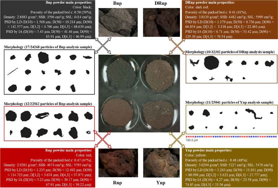
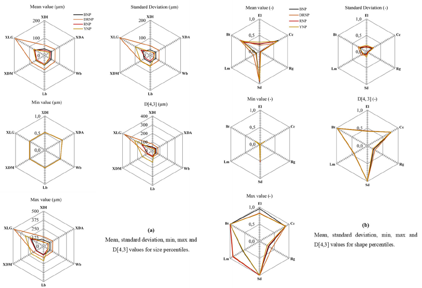
Figure 1: Summary of production process and main testing data of powders.

4 RESULTS AND DISCUSSION

4.1 Principal Properties

The powders obtained have a density between 2.8 and

3.1 g/cm

and SSA Blaine between 3,500 and 5,300

/g, which are comparable to ordinary Portland

cement fineness ((Bouyahyaoui et al, 2018; Juimo et

al, 2017).

By LD, mean particle diameter (Dmed), mean

particle diameter of 10% of particles D(10), median

particle diameter D(50) and mean particle diameter of

90% of particles D(90) were measured to evaluate the

efficiency of the milling process. Using the PSD data

obtain by LD and Equations (1)-(2), 𝑆



evaluated are

ranging between 4,400 to 6,000 cm

/g. 𝑆



value

obtains by this method for each powder is always

higher, that is about 4% to 25% than 𝑆



obtain by BF

(Figure 1).

PSDs of powders were evaluated by using the LD

and IA (Figure 1). In the LD technique, the angular

distribution of light is measured after passing through

an optically dilute dispersion of suspended particles.

This technique is widely used in dust and mineral

industry with water and dispersive agent to a special

cell where the laser light is sent (Felekoglu, 2009;

Orhan et al, 2004).

The inscribed disk diameter (𝑋



or 𝑋



) of each

particle is calculated in real time to build PSD curves

weighted by apparent volume (Gregoire et al, 2007),

making the assumption that particles have identical

flatness ratios, whatever their size (Michel and

Courard, 2014). Area diameter of particles was used

to plot PSD curve obtained by IA. The PSD profile

shows a negligible difference in the results by the two

methods (Abazarpoor et al, 2017). The main reasons

for differences between two PSD methods are as

follows: the considerate particle diameter by each

measurement process, the different shapes of the

particles; better insight into particles using the IA

method; insufficient dispersion of fine particles; fine

particles adhering to the bigger particles. LD and 2D

projection image by the IA are commonly used the

PSD measurement techniques, but the results may not

be representative of the strongly true physical

dimensions of the particles (Califice et al, 2013).

4.2 Particle Morphology Analysis

More than 50 images of powder particles were

identified. The particle morphology was found to

provide reasonable accuracy for estimating the

particle sizes of highly porous particles, where the

distinction between inter-particle and intra-particle

porosity was made. This important comment

concerning inter-particle and intra-particle porosity

has been also reported by Klemm and Wiggins

(Klemm and Wiggins, 2017).

4.2.1 Particle Morphology: Size Parameters

Distribution

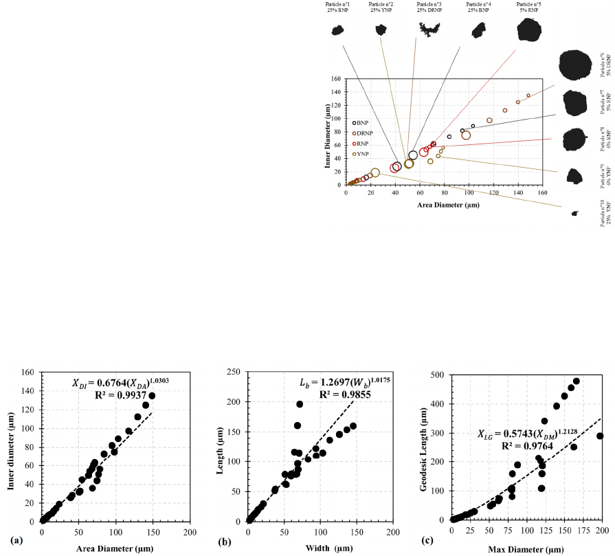
Figure 2 shows the general identification of particles

according to their inner diameter and area diameter.

About 25% of Bnp particles, 25% of Ynp particles,

25% of DRnp particles, 25% of Bnp and 5% of Bnp

particles have the same area diameter like

respectively a particle n°1, n°2, n°3, n°4 and n°5 as

showing in Figure 2. In the same way, about 5% of

DRnp particles, 5% of Bnp particles, 6% of Rnp

particles, 6% of Ynp and 25% of Ynp particles have

the same area diameter like respectively a particle

n°1, n°2, n°3, n°4 and n°5 as showing in Figure 2.

Figure 2: Identification of particles based on their inner

diameter and area diameter.

Particles who have a high inner diameter and area

diameter are from DRnp powder and Particles who

present a very few inner diameter and area diameter

are from Rnp and Ynp powders.

Figure 3: Relation between (a) inner and area diameter, (b) width and length and (c) max distance and geodesic length consider

all powders.

Figure 3a shows that for all data obtained for all

powders, inner diameter and area diameter are well

related with a coefficient of correlation up to 0.99.

Figure 4 shows the general identification of

particles according to their inner diameter and area

diameter. About 25% of Bnp particles, 25% of DRnp

particles, 25% of Bnp particles, 6% of Ynp and 5% of

Bnp particles have the same width as particles n°11,

n°12, n°13, n°9 and n°7 respectively as shown in

Figure 4.

In the same way, about 5% of DRnp particles, 5%

of Rnp particles, 25% of Rnp particles, 25% of Rnp

and 25% of Ynp particles have the same length as

particles n°6, n°14, n°8, n°15 and n°16 respectively

as also shown in Figure 4. Particles that have a higher

width are from DRnp powder and those that present a

higher length are from Ynp powder. Particles that

present a very few width and length are from Rnp and

Ynp powders. Figure 3b shows that for all data

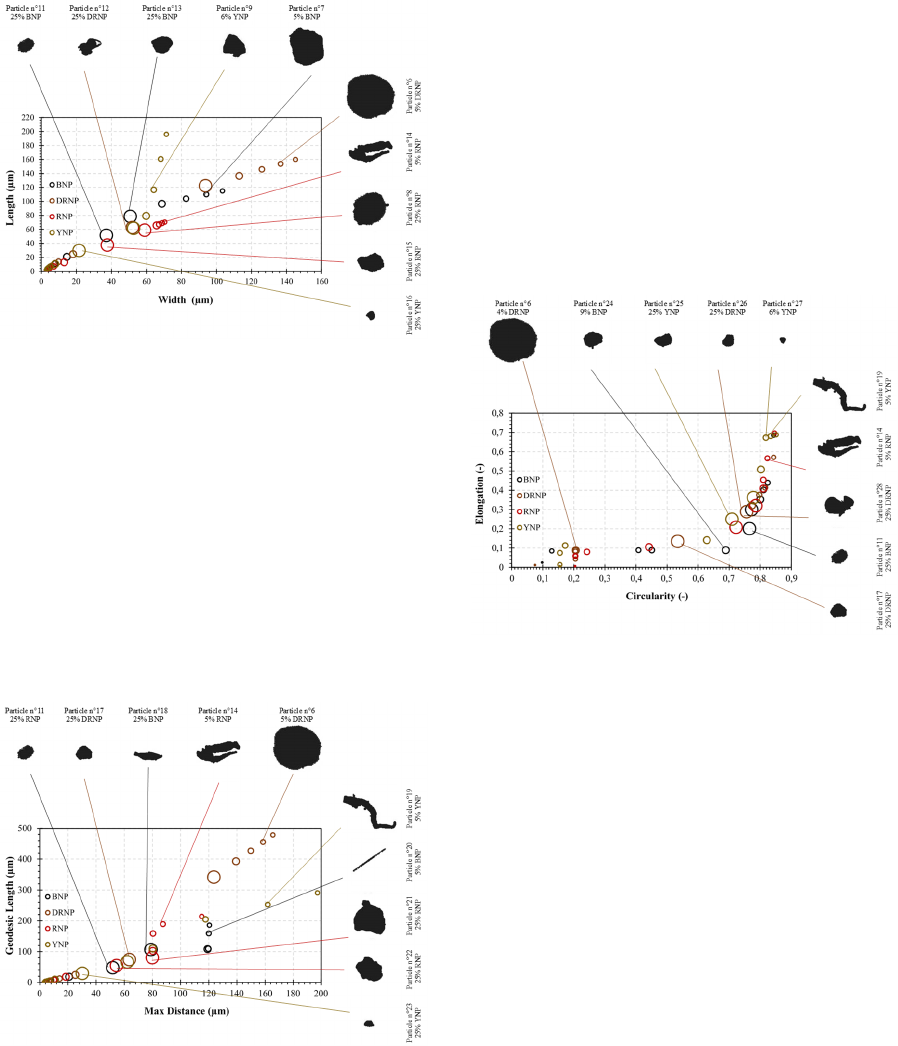
obtained for all powders, width and length are well

related with a coefficient of correlation up to 0.98.

Figure 4: Identification of particles based on their width and

length.

Figure 5 shows the general identification of

particles according to their max distance and geodesic

length. About 25% of Bnp particles, 25% of DRnp

particles, 25% of Bnp particles, 5% of Rnp and 5% of

DRnp particles have the same max distance as

particles n°11, n°17, n°18, n°14 and n°6 respectively

as shown in Figure 5. In the same way, about 5% of

Ynp particles, 5% of Bnp particles, 25% of Rnp

particles, 25% of Rnp and 25% of Ynp particles have

the same geodesic length as particles n°19, n°20,

n°21, n°22 and n°23 respectively as also shown in

Figure 5.

Figure 5: Identification of particles based on their max

distance and geodesic length.

Particles that have a higher max distance are from

DRnp and Ynp powders and whose who present a

higher geodesic length are from DRnp powder.

Particles that present a very few max distance and

geodesic length are from Rnp and Ynp powders.

Figure 3c shows that for all data obtained for all

powders, max distance and geodesic length are well

related with a coefficient of correlation up to 0.97.

4.2.2 Particle Morphology: Shape

Parameters Distribution

Figure 6 shows the general identification of particles

according to their elongation and circularity. About

4% of DRnp particles, 9% of Bnp particles, 25% of

Ynp particles, 25% of DRnp and 6% of Ynp particles

have the same circularity as particles n°6, n°24, n°25,

n°26 and n°27 respectively as shown in Figure 6.

Figure 6: Identification of particles based on their

elongation and circularity.

In the same way, about 5% of Ynp particles, 5%

of Rnp particles, 25% of DRnp particles, 25% of Bnp

and 25% of DRnp particles have the same elongation

as particles n°19, n°14, n°28, n°11 and n°17

respectively as also shown in Figure 6. Particles that

have a higher elongation are from Rnp and Ynp

powders and those that present a higher circularity are

from Rnp and Ynp powders. Particles that present a

very few elongation and circularity are from Bnp and

DRnp powders.

Figure 7 shows the general identification of

particles according to their roughness and solidity.

About 6% of Bnp particles, 6% of DRnp particles, 5%

of DRnp particles, 5% of Rnp and 6% of Ynp

particles have the same roughness as particles n°29,

n°30, n°31, n°32 and n°19 respectively as shown in

Figure 7.

In the same way, about 25% of Rnp particles, 25%

of DRnp particles, 25% of Ynp particles, 25% of Bnp

and 25% of DRnp particles have the same solidity as

particles n°33, n°17, n°25, n°7 and n°6 respectively

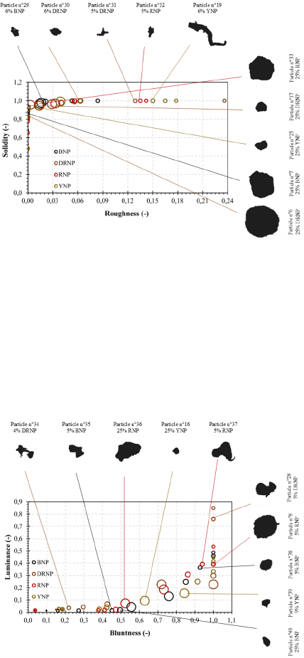
as also shown in Figure 7. Particles that have a higher

roughness are from Ynp powder. Particles that

present a very few roughnesses are also from Ynp

powder. These powder particles have in general a

solidity value equal to 1.0. This means that these

particles from volcanic scoria have a higher solidity.

Figure 7: Identification of particles based on their

roughness and solidity.

Figure 8 shows the general identification of

particles according to their luminance and bluntness.

About 4% of DRnp particles, 5% of Bnp particles,

25% of Rnp particles, 25% of Ynp and 5% of Rnp

particles have the same bluntness as particles n°34,

n°35, n°36, n°16 and n°37 respectively as shown in

Figure 8.

Figure 8: Identification of particles based on their

luminance and bluntness.

In the same way, about 5% of DRnp particles, 5%

of Rnp particles, 5% of Bnp particles, 9% of Ynp and

25% of Bnp particles have the same luminance as

particles n°28, n°8, n°38, n°39 and n°40 respectively

as also shown in Figure 8. Particles that have a higher

luminance are from DRnp powder. Particles that

present a very few luminance are from Rnp and Bnp

powders.

4.3 Study the Correlation Between

Several Parameters

In this study, the two major input systems within

volcanic scoria powder particle morphology (i.e., size

and shape input systems) were compared for their

accuracy in predicting considered dependent variable.

In addition, the effect of number of particle

projections (𝑁



) on the variables obtained through IA

is investigated.

The bestfit models were identified under each

input system. By removing significantly correlated

IPVs within each input system, the regression

modelling process was rerun by shortlisting (Jin et al,

2018).

Figure 9 presents the summary of measurement

values for size and shape parameters of powder

sample identifying the variables considered in this

study. These data are used for the definition of several

models, to predict the considerable dependent

variable. These values have obtained the

consideration of 24,268, 32,302, 22,562 and 25,041

particles for Bnp, DRnp, Rnp and Ynp respectively.

For all size parameters, the value is down to 500 µm

for all powders.

The regression analysis was conducted based on

the proposed models for input systems, respectively.

The reliability of these models was compared, and the

best-fit model was identified. Table 3 displays the

corresponding R

values for all predictions. The

summary of models is shown in Table 3 where the

statistical coefficients analyzed are presented to

evaluate the validity of the regression model. The

model proposed for samples leads a correlation

coefficient (R) of 0.810 and a determination

coefficient (R

) of 0.779, thus revealing a very strong

correlation between the values predicted by the model

and the values observed in the dataset.

Table 3 shows also the analysis of variance

(ANOVA) of models. The ANOVA table reveals an

F value (Fisher-Snedecor test) of models, which is

considerably higher than the critical value of F, for a

level of significance of 5%. Moreover, the

significance value of the model is practically null,

thus lower than the p-value adopted as significance

level (5%). The results obtained reveal that all the

independent variables considered are statistically

significant in explaining the dependent variable.

As shown in Table 3, input systems led to highly

consistent R

values (up to 0.919) from Models 1 to 8

for predicting 𝑋



and 𝑋



, meaning similar

prediction accuracy. Model 4 (the mixed model using

size/shape as the RRV) achieved the consistently high

values for all the four predicted variables (𝑋



𝑋



, 𝑃𝑟



or 𝑃𝑟



Figure 9: Summary of measurement values for size and shape parameters of powders.

All of the corresponding R

values in the 25

scenarios are within the reasonable range (i.e., 0.810–

0.998). Model 1 also achieved the highest R

value

for the prediction of 𝑋



in both systems (0.998 for

Multi-linear regression analysis and 0.979 for Non-

linear model involving variables interactions).

In the 𝑃𝑟



or 𝑃𝑟



regression analysis, Model 6

(the non-linear approach) represents the best-fit

model by achieving even higher accuracy than others,

the highest based on both input systems.

The remaining mixed models had relatively lower

values for both input systems. The R

values

resulting from the best-fit non-linear and mixed

regression models in this research (ranging from

0.810–0.998) are significantly higher than the values

generated from previous studies adopting linear

methods. This can be seen in Table 3.

According to these correlation and ANOVA

coefficients, model 2, model 5 and model 6 are the

three best models to predict max distance and

geodesic length and the best model to predict

Powdering ratio index by Blaine and by LD is the

model 6 as indicated in bold in Table 3.

The linear regression coefficients (𝛼



or 𝛽



) of the

proposed models were determinate. All the

independent variables included in the model are

statistically relevant in the description of the

variability of the dependent variable, showing a

significance value lower than the p-value (5%). The

linear regression coefficients of model present a

significance value lower than the p-value (5%),

indicating that all the independent variables are

statistically relevant in the description of the

dependent response n coefficient obtained from this

test technique (Table 4). These significance values

are marked in green and the models selected on this

basis are also marked in bold in Table 4. According

to these p-values, model 2 and model 5 are the two

best models to predict max distance and geodesic

length and the best model to predict Powdering ratio

index by Blaine and by LD is the model 6 as indicated

in bold in Table 4.

Once the statistical relevance of models is

confirmed, Table 5 presents the mathematical

formulation that makes rating estimation of each

dependent response possible.

Table 3: Summary of the multiple linear regression analysis

results (In this table, *Analysis of variance of the model

(ANOVA), **Square of the mean square error (RMSE))

Parameter Correlation ANOVA*

Eq.

Model n° R R

ad. RMSE** F value

value

Equation

(

)

𝑿

𝑫𝑴

0.998 0.996 0.996 3.868045369 2436.723 0.000

𝑿

𝑫𝑴

0.999 0.998 0.997 2.963935818 3325.711 0.000

𝑿

𝑳𝑮

0.972 0.944 0.944 34.390131493 128.921 0.000

Equation (2)

𝑿

𝑫𝑴

0.942 0.888 0.866 21.326295389 40.846 0.000

𝑿

𝑳𝑮

0.959 0.919 0.904 42.540114280 58.587 0.000

𝑷𝒓

𝑺𝑩

0.951 0.904 0.885 0.286212210 48.326 0.000

𝑷𝒓

𝑺𝑳

0.945 0.892 0.871 0.244277238 42.594 0.000

𝑿

𝑫𝑴

0.968 0.936 0.924 16.097413373 75.576 0.000

𝑿

𝑳𝑮

0.969 0.939 0.927 36.948598108 79.335 0.000

𝑷𝒓

𝑺𝑩

0.944 0.891 0.870 0.304327341 42.150 0.000

𝑷𝒓

𝑺𝑳

0.946 0.896 0.876 0.240259398 44.204 0.000

𝑿

𝑫𝑴

0.989 0.979 0.974 9.349541278 234.136 0.000

𝑿

𝑳𝑮

0.980 0.960 0.952 29.887883900 123.964 0.000

𝑷𝒓

𝑺𝑩

0.942 0.888 0.866 0.308774263 40.798 0.000

𝑷𝒓

𝑺𝑳

0.944 0.892 0.871 0.244995796 42.314 0.000

𝑿

𝑫𝑴

0.998 0.996 0.996 3.787558166 1452.888 0.000

𝑿

𝑳𝑮

0.979 0.959 0.951 30.442169551 119.306 0.000

𝑷𝒓

𝑺𝑩

0.931 0.866 0.840 0.337897319 33.220 0.000

𝑷𝒓

𝑺𝑳

0.936 0.876 0.852 0.261645598 36.467 0.000

𝑿

𝑳𝑮

0.973 0.947 0.937 34.388965646 92.379 0.000

𝑷𝒓

𝑺𝑩

0.930 0.864 0.838 0.340304620 32.679 0.000

𝑷𝒓

𝑺𝑳

0.935 0.873 0.849 0.264888669 35.454 0.000

𝑿

𝑫𝑴

0.966 0.934 0.923 16.211425615 86.685 0.000

𝑷𝒓

𝑺𝑩

0.900 0.810 0.779 0.396643132 26.314 0.000

𝑷𝒓

𝑺𝑳

0.903 0.815 0.785 0.315815860 27.153 0.000

According to these equations with higher

correlation (Table 5), including main characteristics of

powders: the particle size, particle shape and

technological properties of powders (density, surface

area, etc.). It is demonstrated that using powders, as

well as the potential areas of their application, strongly

depends on these characteristics. Dimensionless

relationships between particle size and particle shape

can be determined theoretically for simplified, but

realistic, powder particle geometries. These

relationships have important implications for the

interpretation of shape data, and, more fundamentally,

for the selection of grain size(s) for analysis.

5 CONCLUSIONS

This study showed that the size estimation of

particulate material is a complicated matter. The

results highlight the fact that particle size

distributions may not be unique. Different techniques

can give a large range of different parameters which

need to be interpreted correctly. The choice of the

parameters also depends on the purpose of the

research. It is shown that particle shape analysis that

includes the full range of available grain sizes can

contribute not only measurements of particle size and

shape, but also information on size-dependent

densities and specific surface area.

Based on the analysis of particle characteristics,

design of experiment, and analysis of variance

(ANOVA), it can be concluded that: good correlation

was found between the specific surface area measured

by Blaine Permeability Tester and calculated from the

LD and the IA data.

Thus, based on these conclusions, it appears that

the density, specific surface area, granulometry and,

morphology of volcanic scoria powders may be

efficiently estimated from complementary

techniques. This description is absolutely needed for

understanding particles’ behavior in contact with

water when used in cementitious materials.

ACKNOWLEDGEMENTS

The first author would like to thank Mrs. Sophie

Leroy and Mr. Frédéric Michel, GeMMe research

engineers at the University of Liège (Belgium) for

their help in the testing program.

REFERENCES

Abazarpoor, A., Halali, M., Hejazi, R., Saghaeian, M.,

2017. HPGR effect on the particle size and shape of

iron ore pellet feed using response surface

methodology, Mineral Processing and Extractive

Metallurgy, pp. 1-9.

Arvaniti, E. C., Juenger, M. C. G., Bernal, S. A., Duchesne,

J., Courard, L., Leroy, S., Provis, J. L., Klemm, A., De

Belie, N., 2015a. Physical characterization methods for

supplementary cementitious materials, Materials and

Structures, 48(11):3675–3686.

Arvaniti, E. C., Juenger, M. C. G., Bernal, S. A., Duchesne,

J., Courard, L., Leroy, S., Provis, J. L., Klemm, A., De

Belie, N., 2015b. Determination of particle size,

surface area, and shape of supplementary cementitious

materials by different techniques, Materials and

Structures, 48(11):3687–3701.

Bagheri, G. H., Bonadonna, C., Manzella, I., Vonlanthen,

P., 2015. On the characterization of size and shape of

irregular particles, Powder Technology, 270:141–153.

Bouglada, M. S., Naceri, A., Baheddi, M., Pereira-de-

Oliveira, L., 2019. Characterization and modelling of

the rheological behaviour of blended cements based on

mineral additions, European Journal of Environmental

and Civil Engineering, pp. 1-18.

Bouyahyaoui, A., Cherradi, T., Abidi, M. L., Tchamdjou,

W. H. J., 2018. Characterization of particle shape and

surface properties of powders from volcanic scoria,

Journal of Materials and Environmental Science,

9(7):2032-2041.

Califice, A., Michel, F., Dislaire, G., Pirard, E., 2013.

Influence of particle shape on size distribution

measurements by 3D and 2D image analyses and laser

diffraction, Powder Technology, 237:67–75.

Dioguardi, F., Mele, D., Dellino, P., 2018. A new one-

equation model of fluid drag for irregularly shaped

particles valid over a wide range of Reynolds number,

J. of Geophysical Res.:Solid Earth, 123:144–156.

EN 196-6., 2010. Methods of testing cement - Part 6:

Determination of fineness, European Standard.

Felekoglu, B., 2009. A new approach to the

characterisation of particle shape and surface

properties of powders employed in concrete industry,

Construction and Building Materials, 23:1154–1162.

Ferraris, C. F., Hackley, V. A., Aviles, A. I., Buchanan, C.

E., 2002. Analysis of the ASTM round-Robin test on

particle size distribution of Portland cement: Phase I,

Report no. 6883. Maryland: National Institute of

Standards and Technology (NISTIR).

Gregoire, M. P., Dislaire, G., Pirard, E., 2007. Accuracy of

size distributions obtained from single particle static

digital image analysis, Proceeding. PARTEC

Conference. Nürenberg, 4p.

Hackley, V. A., Lum, L-S., Gintautas V., Ferraris, C. F.,

2004. Particle size analysis by laser diffraction

spectrometry: application to cementitious powders,

Report no. 7097. Maryland: National Institute of

Standards and Technology (NISTIR).

Ilic, M., Budak, I., Vucinic, M., Nagode, A., Kozmidis-

Luburic, U., Hodolic, J., Puskar, T., 2015. Size and

shape particle analysis by applying image analysis and

laser diffraction-inhalable dust in a dental laboratory,

Measurement, 66:109–117.

Jin, R., Chen, Q., Soboyejo, A. B. O., 2018. Non-linear and

mixed regression models in predicting sustainable

concrete strength, Construction and Building Materials,

170:142–152.

Juimo, W. H. T., Grigoletto, S., Michel, F., Courard, L.,

Cherradi, T., Abidi., M. L., 2017. Effects of various

amounts of natural pozzolans from volcanic scoria on

performance of Portland cement mortars, International

Journal of Engineering Research in Africa, 32:36-52.

Juimo, W., Cherradi, T., Abidi, L., Oliveira, L., 2016.

Characterisation of natural pozzolan of "Djoungo"

(Cameroon) as lightweight aggregate for lightweight

concrete, GEOMATE, 11(27):2782-2789.

Klemm, A. J., Wiggins, D. E., 2017. Particle size

characterisation of SCMs by mercury intrusion

porosimetry, Fizyka Budowli W Teorii I Praktyce Tom

IX, Nr 1-2017, pp 5-12.

Liu, E. J., Cashman, K. V., Rust., A. C., 2015. Optimising

shape analysis to quantify volcanic ash morphology,

GeoResJ, 8:14–30.

Michel, F., Courard, L., 2014. Particle size distribution of

limestone fillers: granulometry and specific surface

area investigations, Particulate Science and

Technology, 32:334-340.

Mikli, V., Käerdi, H., Kulu, P., Besterci, M., 2001.

Characterization of powder particle morphology,

Proceedings of the Estonian Academy of Sciences,

Engineering 7(1):22–34.

Neves, R., Silva, A., De Brito, J., Silva, R.V., 2018.

Statistical modelling of the resistance to chloride

penetration in concrete with recycled aggregates,

Construction and Building Materials, 182 : 550–560.

Niesel, K., 1973. Determination of the specific surface by

measurement of permeability, Materials and Structures,

6(3):227-231.

Orhan, M., Özer, M., Işık, N., 2004. Investigation of laser

diffraction and sedimentation methods which are used

for determination of grain size distribution of fine

grained soils, G.U. Journal of Science, 17(2):105–113.

Pavlović, M. G., Pavlović, L. J., Maksimović, V. M.,

Nikolić, N. D., Popov, K. I., 2010. Characterization

and morphology of copper powder particles as a

function of different electrolytic regimes, International

Journal of Electrochemical Science, 5:1862–187.

Slinker, B. K., Glantz, S.A., 2008. Multiple linear

regression: accounting for multiple simultaneous

determinants of a continuous dependent variable,

Circulation, 117(13):1732–1737.

Tchamdjou, W. H. J., Abidi, M. L., Cherradi, T., De

Oliveira, L. A. P., 2017a. Effect of the color of natural

pozzolan from volcanic scoria on the rheological

properties of Portland cement pastes, Energy Procedia,

139:703–709. DOI: 10.1016/j.egypro.2017.11.275.

Tchamdjou, W. H. J., Cherradi, T., Abidi, M. L., De

Oliveira, L. A. P., 2017b. Influence of different amounts

of natural pozzolan from volcanic scoria on the

rheological properties of Portland cement pastes,

Energy Procedia, 139:696–702. DOI:

10.1016/j.egypro.2017.11.274.

Varga, G., Kovács, J., Szalai, Z., Cserháti, C., Újvári, G.,

2018. Granulometric characterization of paleosols in

loess series by automated static image analysis,

Sedimentary Geology, 370, pp 1-14.

Table 4: p-value (In this table, x : non-considered variable, xx : excluded variable).

Model n° Const.

𝑿

𝑫𝑰

𝑿

𝑫𝑨

𝑾

𝒃

𝑳

𝒃

𝑿

𝑫𝑴

𝑿

𝑳𝑮

𝑿

𝑫𝑰

𝑬

𝒍

𝑿

𝑫𝑰

𝑪

𝒄

𝑿

𝑫𝑰

𝑹

𝒈

𝑾

𝒃

𝑺

𝒅

𝑾

𝒃

𝑳

𝒎

𝑾

𝒃

𝑩

𝒕

𝑿

𝑫𝑴

1 0.842 0.226 0.610 0.864 0.000 x x x x x x x x

𝐗

𝐃𝐌

2 0.121 0.001 0.304 0.107 0.000 x 0.000 x x x x x x

𝐗

𝐋𝐆

0.008 0.000 0.030 0.006 0.000 0.000 x x x x x x x

𝑋



3 0.365 x 0.120 x x x x 0.001 0.946 0.038 0.199 0.442 0.203

𝑋



0.289 x 0.046 x x x x 0.969 0.796 0.903 0.034 0.355 0.000

𝑃𝑟



0.279 x 0.405 x x x x 0.584 0.261 0.543 0.234 0.155 0.009

𝑃𝑟



0.160 x 0.287 x x x x 0.863 0.198 0.772 0.159 0.109 0.002

Model 4 Const.

𝑿

𝑫𝑰

𝑿

𝑫𝑨

𝑾

𝒃

𝑳

𝒃

𝑿

𝑫𝑴

𝑿

𝑳𝑮

𝑿

𝑫𝑨

𝑬

𝒍

𝑿

𝑫𝑨

𝑪

𝒄

𝑿

𝑫𝑨

𝑹

𝒈

𝑿

𝑫𝑨

𝑺

𝒅

𝑿

𝑫𝑨

𝑳

𝒎

𝑿

𝑫𝑨

𝑩

𝒕

𝑋



0.365 x 0.120 x x x x 0.001 0.946 0.038 0.199 0.442

0.203

𝑋



0.289 x 0.046

x x x x

0.969 0.796 0.903 0.034

0.355

0.000

𝑃𝑟



0.279 x 0.405

x x x x

0.584 0.261 0.543

0.234 0.155

0.009

𝑃𝑟



0.160 x 0.287

x x x

x 0.863 0.198 0.772 0.159 0.109 0.002

Model 5 Const.

𝑿

𝑫𝑰

𝑿

𝑫𝑨

𝑾

𝒃

𝑳

𝒃

𝑿

𝑫𝑴

𝑿

𝑳𝑮

𝑾

𝒃

𝑬

𝒍

𝑾

𝒃

𝑪

𝒄

𝑾

𝒃

𝑹

𝒈

𝑾

𝒃

𝑺

𝒅

𝑾

𝒃

𝑳

𝒎

𝑾

𝒃

𝑩

𝒕

𝑿

𝑫𝑴

0.110 x x 0.094 x x x 0.000 0.265 0.000 0.042 0.000

0.667

𝑿

𝑳𝑮

0.748 x

x 0.169 x x x 0.000 0.757 0.000 0.105 0.907

0.000

𝑃𝑟



0.334

x x

605

x x 0.885

0.267

0.944 0.358 0.023 0.002

𝑃𝑟



0.118

x x

0.249 x x

x 0.870 0.182 0.462 0.130 0.001 0.001

Model 6 Const.

𝑿

𝑫𝑰

𝑿

𝑫𝑨

𝑾

𝒃

𝑳

𝒃

𝑿

𝑫𝑴

𝑿

𝑳𝑮

𝑳

𝒃

𝑬

𝒍

𝑳

𝒃

𝑪

𝒄

𝑳

𝒃

𝑹

𝒈

𝑳

𝒃

𝑺

𝒅

𝑳

𝒃

𝑳

𝒎

𝑳

𝒃

𝑩

𝒕

𝑋



0.519 x x x 0.966 x x 0.908 0.386 0.330 0.313 0.400

0.384

𝑋



0.783 x x

x 0.261 x x 0.001 0.952 0.084 0.185 0.336

0.000

𝑷𝒓

𝑺𝑩

0.035

x x 0.070 x x 0.041

0.246

0.523 0.042 0.510 0.049

𝑷𝒓

𝑺𝑳

0.012

x x 0.028

x x 0.091 0.183 0.533 0.017 0.260 0.017

Model 7 Const.

𝑿

𝑫𝑰

𝑿

𝑫𝑨

𝑾

𝒃

𝑳

𝒃

𝑿

𝑫𝑴

𝑿

𝑳𝑮

𝑿

𝑫𝑴

𝑬

𝒍

𝑿

𝑫𝑴

𝑪

𝒄

𝑿

𝑫𝑴

𝑹

𝒈

𝑿

𝑫𝑴

𝑺

𝒅

𝑿

𝑫𝑴

𝑳

𝒎

𝑿

𝑫𝑴

𝑩

𝒕

𝑋



0.906 x x x x 0.281 x 0.002 0.931 0.061 0.208 0.603

0.000

𝑃𝑟



0.037 x x x x 0.092 x 0.035 0.325 0.349 0.056 0.371 0.078

𝑃𝑟



0.013 x

x 0.040 x 0.078

0.255 0.352 0.023 0.176 0.030

Model 8 Const.

𝑿

𝑫𝑰

𝑿

𝑫𝑨

𝑾

𝒃

𝑳

𝒃

𝑿

𝑫𝑴

𝑿

𝑳𝑮

𝑿

𝑳𝑮

𝑬

𝒍

𝑿

𝑳𝑮

𝑪

𝒄

𝑿

𝑳𝑮

𝑹

𝒈

𝑿

𝑳𝑮

𝑺

𝒅

𝑿

𝑳𝑮

𝑳

𝒎

𝑿

𝑳𝑮

𝑩

𝒕

𝑋



0.399 x x x x x 0.076 0.010 0.111 0.136 xx 0.390

0.000

𝑃𝑟



0.182

x x

x x x 0.127

0.939 0.021

0.570 xx 0.499

0.000

𝑃𝑟



0.122 x

x x

0.160 0.585

0.011 0.460 xx 0.351 0.000

Table 5: Equations of efficient models identified.

Model n° Equations R

Model 2



 1.167  0.435X



 0.281X



 0.501



 1.043L



 0.056X



0.998



 22.528  6.003X



 6.718X



 9.542



 8.240L



 7.590X



0.944

Model 5



 6.306  4.455



 1.989



E



 0.827



C



 4.877







 5.815



S



 1.377



L



 0.157



B



0.979



 3.989  11.619



 6.019



E



 0.727



C





8.110







 14.650



S



 0.053



L



 7.069



B



0.960

Model 6



 0.302  0.145L



 0.031L



E



 0.024L



C



 0.025L









0.175L



S



 0.006L



L



 0.021L



B



0.866



 0.282  0.137L



 0.019L



E



 0.021L



C



 0.019L









0.162L



S



 0.008L



L



 0.020L



B



0.876