
Application of the Lattice Boltzmann Method to the Acoustic Wave in
a Rectangular Enclosure
Jaouad Benhamou
1a
, Mohammed Jami
1b
and Ahmed Mezrhab
1
1
Mechanics & Energetics Laboratory, Faculty of Sciences, Mohammed First University, 60000 Oujda, Morocco.
Keywords: Lattice Boltzmann method, acoustic waves, analytical solution, absolute error.
Abstract: An application of the lattice Boltzmann method (LBM) to the study of sound wave propagation is presented
in this paper. The major purpose of this simulation is to show how the LBM technique can be easily applied
in the domain of acoustics. The sound waves are emitted from a vibrating rectangular source placed in the
center of the left face of a rectangular enclosure filled with air. An analytical study is performed to validate
our numerical approach and the error between the two studies is also described to ensure the validity of the
LBM analysis.
1 INTRODUCTION
The history of the LBM method stems from two
different approaches, the kinetic theory of discrete
velocity distribution gases and lattice gases
(Bechereau, 2017). The first approach is generally
used to model a system composed of a large number
of particles such as a gas using statistical description
tools (Mohamad, 2011; Timm et al, 2017; Tristani,
2015). A lattice gas is a cellular automaton developed
to simulate the behaviour of a fluid (Frisch et al.,
1986; McNamara and Zanetti, 1988). That is, a
structured grid of cells. Each of these cells is in a state
(empty or full) which evolves over time.
The application of the LBM in different scientific
fields has been well known in the literature for a long
time. This numerical method is a mesoscopic
approach that can simulate various physical
mechanisms such as fluid flows, wave propagation
and heat transfer. For example, for wave simulation,
the LBM has been employed for many years to study
many types of waves such as elastic (Frantziskonis,
2011; O’Brien et al., 2012), sound (Benhamou et al.,
2020; Buick et al., 1998; Salomons et al., 2016),
aeroacoustic (Marié et al., 2009; Weidong and Jun,
2019) and shock waves (Guangwu et al., 1999; Xiao,
2007).
a
https://orcid.org/0000-0002-1958-2843
b
http://orcid.org/0000-0002-5356-4729
In this article, our work deals with numerical and
analytical studies of the sound waves propagation.
For numerical simulation, the LB method is used to
model the waves produced using the point source
modelling tool. In the analytical case, the study will
be carried out using the mathematical expression of
cylindrical waves given by the resolution of the
standing wave equation.
It is important to mention that the study of sound
waves is chosen in this article as a research topic
because its applications are very important in various
fields, especially in the industrial (Moudjed, 2013)
and medical (Ranganayakulu et al., 2016; Sarvazyan
et al., 2013) sectors.
2 NUMERICAL APPROACH
For the LBM simulations, there are two popular
models to simulate different physical problems:
multiple relaxation time (MRT) and single relaxation
time (SRT) models. In the case of acoustic wave
simulation, the MRT model is more stable and precise
than the SRT scheme (Viggen, 2009). For this simple
reason, the LBM-MRT model is chosen in this work
to simulate the wave propagation. In this way, the
description of the fluid evolution using this model can
be given by the following discrete Boltzmann
equation (Mohamad, 2011; Benhamou et al., 2020;
Jami et al., 2016; Mezrhab et al., 2010):
𝑓
𝑥
𝑐
𝛥𝑡, 𝑡 𝛥𝑡
𝑓
𝑥
,𝑡
𝑀
𝑆𝑚
𝑚
where 𝑓
represents the distribution function in
direction 𝑖, 𝑐
denotes the velocities of the lattice used,
𝛥𝑡 is the time step, 𝑆 is the relaxation matrix and 𝑀
is the inverse matrix of the transformation matrix 𝑀.
𝑚
and 𝑚
are the fluid moments and equilibrium
moments, respectively.
The discretization of the velocity space allows to
define the LBM lattice. Therefore, it is necessary to
choose a set of well reduced velocities to optimize the
computation time of the LBM simulations. However,
the number of velocities must be sufficient to describe
the dynamic behaviour of the flow and the velocities
should not be chosen randomly. The choice of the
LBM lattice is therefore very important. Generally, it
is necessary to choose a symmetrical lattice in order
to obtain the flow behaviour at the macroscopic scale.
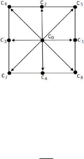
Usually, the D2Q9-LBM scheme (Figure 1) is
employed to determine the macroscopic quantities
such as velocities and density (Mohamad, 2011).
Figure 1: The D2Q9-LBM model.
The matrix 𝑆 is a diagonal matrix. In this LBM
simulation, the nine relaxation rates are the same as
those mentioned in the references (Mohamad, 2011;
Benhamou et al., 2020):
Sdiag
1,1.4,1.4,1,1.2,1,1.2,𝑠
,𝑠
(2)
The two relaxation rates s
and s
are equal and
related to the kinematic viscosity (ν) as:
s
s
.
(3)
The matrices 𝑀 and 𝑀
are matrices (9*9). Their
role is to map the nine distribution functions to the
space of moments:
𝑚𝑀𝑓 and 𝑓𝑀
𝑚 (4)
The mathematical expression of the M is given as
(Mohamad, 2011):
𝑀
⎝
⎜
⎜
⎜
⎜
⎜
⎜
⎜
⎛
111111111
010101111
0 0 1 0 1 1 1 1 1
4 1 1 1 1 2 2 2 2
422221 1 1 1
02 0 2 0111 1
0 0 2 0 2 1 1 1 1
0 11 110 0 0 0
000001111
⎠
⎟
⎟
⎟
⎟
⎟
⎟
⎟
⎞
(5)
The moment vector 𝑚 is given as a function of the
density, physical energy, energy flux, impulsion and
the physical quantities related to the components of
the stress tensor (Benhamou et al., 2020; Mezrhab et
al., 2010).
The vector 𝑚
depends of the fluid density and
the macroscopic velocities (𝑢,𝑣) (Mohamad, 2011).
𝑚
𝜌
𝑚
2𝜌3𝜌
𝑢
𝑣
𝑚
𝜌3𝜌
𝑢
𝑣
𝑚
𝜌𝑢
𝑚
𝜌𝑢 (6)
𝑚
𝜌𝑣
𝑚
𝜌𝑣
𝑚
𝜌
𝑢
𝑣
𝑚
𝜌
𝑢𝑣
Differently from CFD methods, which are based
on solving the differential equations, the LBM is a
statistical approach that gives the macroscopic
quantities as the mean of the microscopic quantities
outlined by the functions 𝑓
. For example, for the
D2Q9 schema, the density (𝜌) and velocities (𝑢,𝑣
)
can be computed as (A. A. Mohamad, 2011):
𝜌
∑
𝑓
, 𝜌𝑢
∑
𝑓
𝑐
and 𝜌𝑣
∑
𝑓
𝑐
(7)
where 𝑐
are the nine LBM velocities of the D2Q9
model.
3 BOUNDARY CONDITIONS
The boundary conditions applied at all walls of the
rectangular enclosure are the bounce-back boundary
conditions (BBC). These types of conditions are
typically employed to rebound the fluid particles at
the solid boundaries. The BBC are based on the idea
that the known functions can be exploited at the
boundaries to determine the unknown functions. For
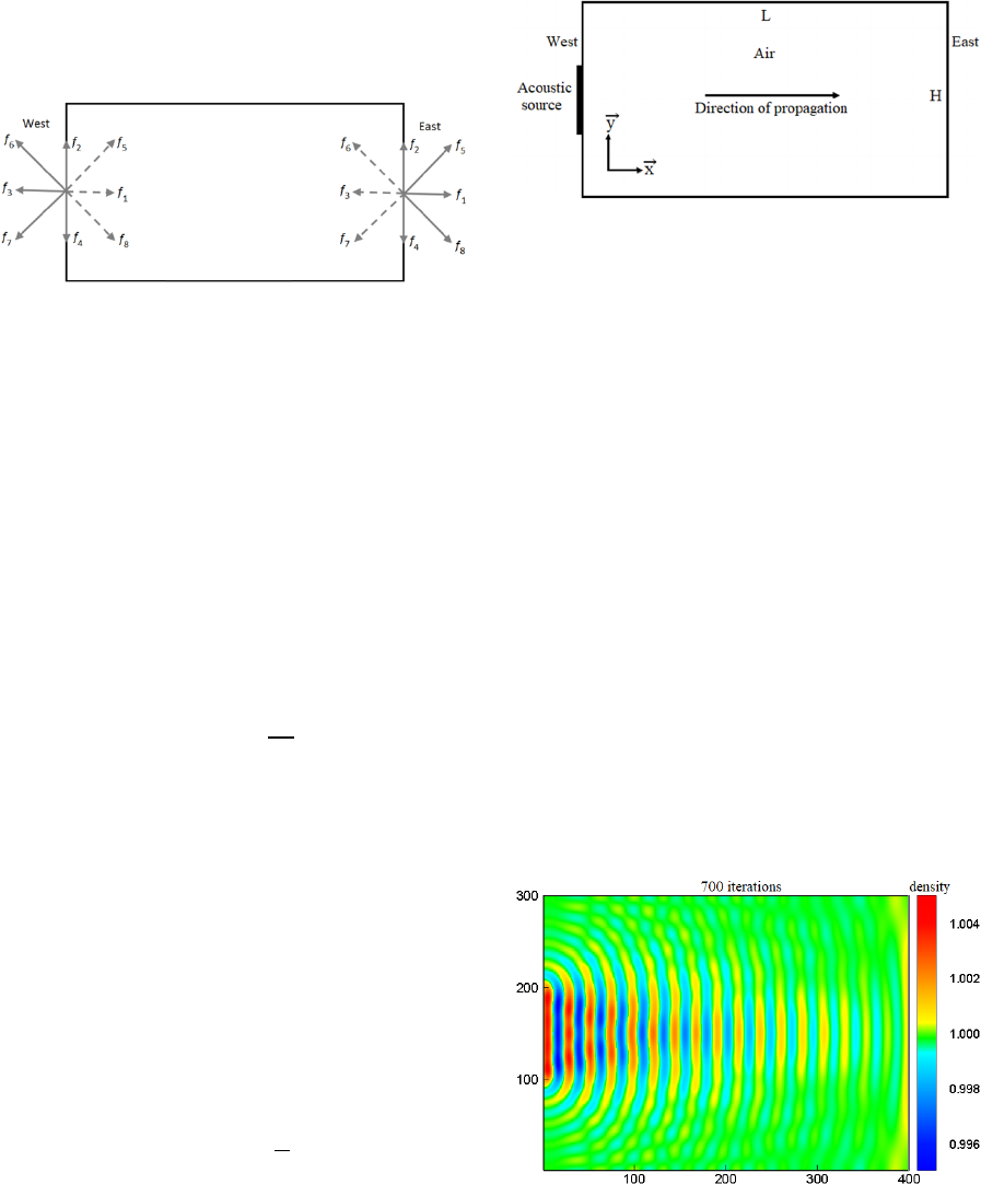
example, an implementation of the BBC at the
vertical walls of a rectangular cavity is illustrated in
figure 2. At the west boundary, the functions 𝑓
, 𝑓
and 𝑓
are respectively replaced by 𝑓
, 𝑓
, 𝑓
. At the
east wall, the functions 𝑓
, 𝑓
and 𝑓
are given as
follows: 𝑓
𝑓
, 𝑓
𝑓
and 𝑓
𝑓
.
Figure 2: Illustration of the Bounce-back boundary
conditions.
4 RESULTS AND DISCUSSION
The geometry of the physical problem is depicted in
figure 3. The sound waves are emitted by a vibrating
rectangular source placed in the center of the left wall
of a rectangular enclosure filled with air. The acoustic
source is discretized into a set of point sources based
on the acoustic point source technique (Benhamou et
al., 2020; Salomons et al., 2016; Viggen, 2009). This
technique allows the sound waves to be easily
produced. For a single point source, the waves can be
described by the following equation:
𝜌𝜌
𝜌
𝑠𝑖𝑛
(8)
where the parameters 𝜌
, 𝑡, 𝑇 and 𝜌
represent the
amplitude, the time, the period, and the equilibrium
density (𝜌
1), respectively.
It should be noted that this model is only valid in
cases of weak oscillations, i.e. in cases where the
amplitude is very small compared to the equilibrium
density ( 𝜌
≫𝜌
) (Viggen, 2009).
For the point source, it is necessary to confirm
that it behaves in a way that corresponds to the
analytical solution of the simulated physical problem.
In 2D, the emitted acoustic waves are the circular
waves corresponding to the cylindrical waves in 3D
(Salomons et al., 2016; Viggen, 2009). Thus, the
analytical solution can be expressed as:
𝜌
𝐴𝐻
𝑘𝑟
𝑒
(9)
where 𝐴 is a constant, 𝐻
is the Hankel function,
which depends on the wave number 𝑘 and the
distance to the source 𝑟 . All the parameters
represented in this equation (Equation (9)) are well
discussed in the references (Benhamou et al., 2020;
Viggen, 2009).
Figure 3: Simulated physical problem.
It should be noted that our LBM code has already
been validated by comparing our results obtained
from a single acoustic source placed in the center of a
square air-filled cavity. This validation is illustrated
in reference (Benhamou et al., 2020). It is reported on
the simulation of circular wave propagation in air at
time 1600 and for a period and viscosity of 40 and
0.06, respectively.
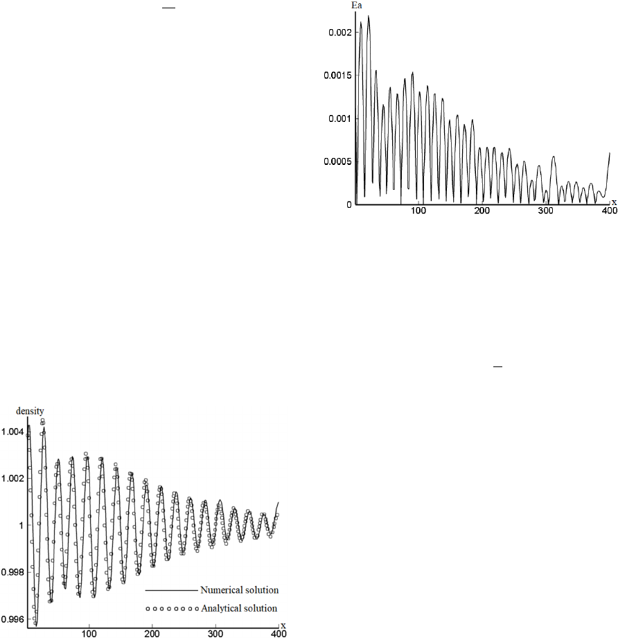
The numerical results obtained for this simulation
are given in figure 4 . From this figure, it can be seen
that the waves produced are plane and propagating in
the x-direction towards the right wall of the enclosure.
These waves are obtained by the interference of
circular waves emitted by discrete acoustic point
sources. This result are obtained at 700 iterations
(𝑡700). At this time, the waves arrive at the east
wall and begin to be reflected by this boundary.
The diameter of the rectangular source considered
here is H/3, it corresponds to 100 point sources for a
mesh of 400*300 nodes. The priode (𝑇) is equal to 40,
the viscosity () is fixed at 0.02 and the amplitude
(𝜌
) is chosen in a way that the acoustic model used
always remains linear (𝜌
0.01) (Benhamou et al.,
2020).
Figure 4: Simulation results of the acoustic waves
propagation in enclosure filled with air at 700 iterations.
To further validate our numerical results, the
analytical analysis results are also presented in this
work. As mentioned previously, for a single acoustic
source, this analytical solution is given by equation
(9). In the case of the source shown in figure 3, the
analytical solution is given by the sum of the density
fields of the point acoustic sources.
The mathematical expression of the constant 𝐴
appearing in equation (9) can be expressed as
(Viggen, 2009) :
𝐴𝑎 𝜌
𝑒
(10)
where 𝑎 is a constant and 𝜌
is the amplitude of the
point source. The factor 𝑎 depends in particular on
the viscosity used. For example, for a LBM period of
20, the values of 𝑎 found by Viggen (Viggen, 2009)
for viscosities of 0.166 and 0.033 are 0.135 and 0.15,
respectively.
It is worth noting that the mathematical
expression of 𝐴 (equation (10)) is given from a
comparison of the analytical and numerical results
(Viggen, 2009). The analytical resolution of equation
(9) gives an analytical solution very close to the
numerical results found. However, there is a
discrepancy (gap) between these two solutions. This
is due to the term 𝑒
/
expressed in equation (10).
This gap can be clearly seen in figure 5, which
represents the analytical and numerical longitudinal
profiles of the density along the x-axis at time 700 and
at the position H/2. The calculation of the absolute
error ( Ea ) is also presented. This error can be
determined as the difference between the analytical
(𝜌
) and numerical (𝜌
) densities (Benhamou et
al., 2020):
𝐸𝑎
|
𝜌
𝜌
|
(11)
Figure 5: Longitudinal profiles of the numerical and
analytical densities along the x-axis given by equations (8)
and (9) in the presence of the constant 𝐴 expressed in
equation (10).
Figure 6 illustrates the variation of 𝐸𝑎 along the
x-axis. It fluctuates between 0 and 2.22 10
very
close to the rectangular sound source and its variation
becomes small away from the source. It should be
noted that for the maximum value found in this
calculation (2.22 10
), the error can be considered
significant in relation to the variation of the density,
which oscillates between 0.996 and 1.004 (see Figure
5). Consequently, the analytical solution must be
improved.
Figure 6: Fluctuation of the absolute error between the
analytical and numerical densities along the x-axis.
Many tests have been performed to improve the
gap between analytical and numerical results, i.e. to
improve the absolute error. We found very good
agreement between the two results if equation (10)
becomes:
𝐴𝑎 𝜌
𝑒
(12)
It is important to note that the absolute value of
the density obtained by using this last expression is
high compared to that found by using equation (10)
and therefore it leads to the improvement of the
absolute error between the numerical and analytical
results. The change of the mathematical expression of
the constant A is tested in the present studied
configuration and will be tested in other subsequent
work. The new results found are shown in figure 7. A
good correspondence between the analytical and
numerical calculations can be seen from this figure.
As for the first case, the absolute error (Ea) is
calculated and is depicted in figure 8. From this
figure, it can be seen that Ea varies between 0 and
about 4.5 10
along the x-axis, except in the vicinity
of the acoustic source and the right wall of the cavity
where it takes a more significant value. The
maximum value of Ea (8 10
) can be considered
very low compared to its former maximum value
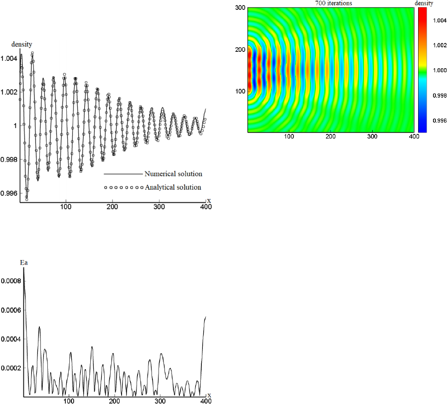
( 2.22 10
) which indicates that the numerical
results are now very close to those calculated
analytically.
Figure 7: Longitudinal profiles of the analytical and
numerical densities found after the improvement of the
mathematical expression of the constant A (equation (12)).
Figure 8: Oscillation of the absolute error between the
analytical and numerical densities along the x-axis after the
improvement of the mathematical expression of the
constant A (equation (12)).
The analytical density field is shown in figure 9,
in order to compare it with the numerical result shown
in figure 4. There is a good resemblance between the
two figures. Note, however, that due to the reflection
of the waves due to the bounce-back boundary
conditions applied in the numerical calculations,
interferences occur and modify the waveform near the
walls with regard to the analytically calculated
density field. The reflected waves can be absorbed
using the absorption boundary conditions, and this
will be a future study.
Figure 9: Analytical results found using the sum of the
density expressed in equation (9) in the presence of the
constant 𝐴 formulated in equation (12).
5 CONCLUSIONS
This work deals with the simulation of acoustic waves
using the MRT-LBM method. The numerical study
presented here has shown that the LB method can be
used to simulate the acoustic waves generated in air
by a rectangular acoustic source. The proposed
numerical model presents a good accuracy, confirmed
by the comparison with the analytical calculation that
is improved in this study compared to the one already
reported in the literature. This validation is carried out
using the mathematical expression of the density
given by the wave equation solution for the case of
cylindrical waves emitted by point sources
(Benhamou et al., 2020).
REFERENCES
Bechereau, M. (2016). Élaboration de méthodes Lattice
Boltzmann pour les écoulements bifluides à ratio de
densité arbitraire (Doctoral dissertation).
Timm, K., Kusumaatmaja, H., Kuzmin, A., Shardt, O.,
Silva, G., and Viggen, E. (2016). The lattice Boltzmann
method: principles and practice. Springer International
Publishing AG Switzerland, ISSN, 1868-4521.
Mohamad, A. A. (2011). Lattice Boltzmann Method (Vol.
70). London: Springer.
Tristani, I. (2015). Existence et stabilité de solutions fortes
en théorie cinétique des gaz (Doctoral dissertation,
Paris 9).
Frisch, U., Hasslacher, B., and Pomeau, Y. (1986). Lattice-
gas automata for the Navier-Stokes equation. Physical
review letters, 56(14), 1505.
McNamara, G. R., and Zanetti, G. (1988). Use of the
Boltzmann equation to simulate lattice-gas
automata. Physical review letters, 61(20), 2332.

Frantziskonis, G. N. (2011). Lattice Boltzmann method for
multimode wave propagation in viscoelastic media and
in elastic solids. Physical Review E, 83(6), 066703.
O’Brien, G. S., Nissen‐Meyer, T., and Bean, C. J. (2012).
A lattice Boltzmann method for elastic wave
propagation in a poisson solid. Bulletin of the
Seismological Society of America, 102(3), 1224-1234.
Buick, J. M., Greated, C. A., and Campbell, D. M. (1998).
Lattice BGK simulation of sound waves. EPL
(Europhysics Letters), 43(3), 235.
Salomons, E. M., Lohman, W. J., and Zhou, H. (2016).
Simulation of sound waves using the lattice Boltzmann
method for fluid flow: Benchmark cases for outdoor
sound propagation. PloS one, 11(1), e0147206.
Benhamou, J., Jami, M., Mezrhab, A., Botton, V., and
Henry, D. (2020). Numerical study of natural
convection and acoustic waves using the lattice
Boltzmann method. Heat Transfer, 49(6), 3779-3796.
Marié, S., Ricot, D., and Sagaut, P. (2009). Comparison
between lattice Boltzmann method and Navier–Stokes
high order schemes for computational
aeroacoustics. Journal of Computational
Physics, 228(4), 1056-1070.
Weidong, S. H. A. O., and Jun, L. I. (2019). Review of
Lattice Boltzmann Method Applied to Computational
Aeroacoustics. Archives of Acoustics, 44(2), 215-238.
Guangwu, Y., Yaosong, C., and Shouxin, H. (1999). Simple
lattice Boltzmann model for simulating flows with
shock wave. Physical review E, 59(1), 454. Guangwu,
Y., Yaosong, C., & Shouxin, H. (1999). Simple lattice
Boltzmann model for simulating flows with shock
wave. Physical review E, 59(1), 454.
Xiao, S. (2007). A lattice Boltzmann method for shock
wave propagation in solids. Communications in
numerical methods in engineering, 23(1), 71-84.
Moudjed, B. (2013). Caractérisation expérimentale et
théorique des écoulements entrainés par ultrasons.
Perspectives d'utilisation dans les procédés de
solidification du silicium photovoltaïque (Doctoral
dissertation, Lyon, INSA).
Sarvazyan, A. P., Urban, M. W., and Greenleaf, J. F.
(2013). Acoustic waves in medical imaging and
diagnostics. Ultrasound in medicine & biology, 39(7),
1133-1146.
Ranganayakulu, S. V., Rao, N. R., and Gahane, L. (2016).
Ultrasound applications in medical
sciences. IJMTER, 3, 287-93.
Viggen, E. M. (2009). The lattice Boltzmann method with
applications in acoustics (Master's thesis, Norges
teknisk-naturvitenskapelige universitet, Fakultet for
naturvitenskap og teknologi, Institutt for fysikk).
Mezrhab, A., Moussaoui, M. A., Jami, M., Naji, H., and
Bouzidi, M. H. (2010). Double MRT thermal lattice
Boltzmann method for simulating convective
flows. Physics Letters A, 374(34), 3499-3507.
Jami, M., Moufekkir, F., Mezrhab, A., Fontaine, J. P., and
Bouzidi, M. H. (2016). New thermal MRT lattice
Boltzmann method for simulations of convective
flows. International Journal of Thermal Sciences, 100,
98-107.
