Time-series Modeling for Consumer Price Index Forecasting using
Comparison Analysis of AutoRegressive Integrated Moving Average
and Artificial Neural Network
Intan Yuniar Purbasari
1
, Fetty Tri Anggraeny
1
and Nindy Apsari Ardiningrum
2
1
Department of Informatics, Faculty of Computer Science, Universitas Pembangunan Nasional “Veteran” Jawa Timur,
Raya Rungkut Madya, Surabaya, Indonesia
2
Alumni of Department of Informatics, Faculty of Computer Science, Universitas Pembangunan Nasional “Veteran” Jawa
Timur
Keywords: ARIMA, ANN, Consumer Price Index, Time Series Data
Abstract: The Consumer Price Index (CPI) is an index number that measures the average price of goods consumed by
households and is one factor that influences inflation in a country. The CPI forecast is calculated in monthly
periods each year to anticipate the possibility of a spike in the inflation rate. Forecasting the CPI makes use
of past values, commonly known as time-series data (TSD). One method to assist the forecasting process on
TSD is the Autoregressive Integrated Moving Average (ARIMA). However, ARIMA is less accurate for
nonlinear data problems. Another method that can also be used for forecasting with linear data problems is
the Artificial Neural Network (ANN). This study compared the two forecasting methods between ARIMA
and ANN by predicting the Indonesian CPI value from January - December 2018. The TSD used is in data
on the Indonesian CPI value between January 2009 and December 2017. This study indicates that the ANN
method is better than ARIMA because it produces a smaller MSE of 59.23. However, ARIMA is also good
because the two methods' forecast results are in the range of the CPI value.
1 INTRODUCTION
In economic terms, inflation is a term that
significantly affects the economy of a country,
which is a process of increasing prices for both
goods and services continuously during a specific
period measured using a price index (Nopirin, 1987).
One of the most frequently used price indexes to
measure inflation is the Consumer Price Index
(CPI). CPI compares prices in a month against the
previous month, which is based on the base year for
calculating the CPI. The effect on inflation is that
the higher the resulting index value, the greater the
possibility of inflation. In one condition, inflation
can be considered beneficial, but it can also be
regarded as detrimental. But in general, inflation can
lead to economic instability, failure to carry out
development, and lower levels of living and welfare.
Monthly CPI values may be predicted for the
next several periods using statistical analysis. CPI
forecasting can be made with one of the forecasting
methods that use time-series data, including
AutoRegressive Integrated Moving Average
(ARIMA), AutoRegressive Fractionally Integrated
Moving Average (ARFIMA), Winter,
Autoregressive Conditional Heteroskedasticity
(ARCH), and other algorithms (Wigati, Rais, &
Utami, 2016). However, in general, economic data
forecasting such as CPI, mostly uses the ARIMA
method (Pimpi, 2013) (Deswina & Desmita, 2015),
(Wigati, Rais, & Utami, 2015), (Mohamed, 2020).
This is because the ARIMA method is sufficient for
short-term forecasting, whereas if used for long-term
forecasting, the resulting value will tend to be
constant (Djawoto, 2010). In (Hiteshi Tandon, 2020)
a model has been developed to forecast future
COVID-19 cases in India using ARIMA based time-
series analysis. ARIMA is also successful in
predicting stock price which is a short term
prediction (Adebiyi, Adewumi, & Ayo, 2014).
According to (Janah, Sulandari, & Wiyono, 2014),
the ARIMA model is a time series modeling for
linear data, but in reality, not all phenomena that use
time series have a linear relationship. Instead, some
are nonlinear. Therefore, we also need a method that
Purbasari, I., Anggraeny, F. and Ardiningrum, N.
Time-series Modeling for Consumer Price Index Forecasting using Comparison Analysis of AutoRegressive Integrated Moving Average and Artificial Neural Network.
DOI: 10.5220/0010369200003051
In Proceedings of the International Conference on Culture Heritage, Education, Sustainable Tourism, and Innovation Technologies (CESIT 2020), pages 599-604
ISBN: 978-989-758-501-2
Copyright
c
 2022 by SCITEPRESS – Science and Technology Publications, Lda. All rights reserved
599

can solve nonlinear problems. One such approach is
the Artificial Neural Network (ANN) (Fitriani,
Ispriyanti, & Prahutama, 2015), which is a system
utilized by modeling the workings of the human
brain neural network to complete calculation forms
(Susilokarti, Arif, Susanto, & Sutiarso, 2015).
Similar approach was also proposed by (Domingos
S. de O. Santos Júnior, 2019) which evaluated the
use of hybrid systems of ARIMA combined with
Multilayer Perceptron and Support Vector Machine,
while (Ümit Çavuş Büyükşahin, 2019) used
ARIMA-ANN hybrid method improved by
Empirical Mode Decomposition.
This study compared two forecasting methods,
ARIMA and ANN, to predict the Indonesian CPI
with time-series data for January 2009 - August
2018 and assessed the accuracy of forecasting based
on the MSE criteria and the calculation of the CPI
value range.
2 MATERIALS AND METHOD
2.1 Dataset
Dataset used is a secondary data on the Indonesian
Consumer Price Index (CPI), which is quantitative
starting from January 2009 - December 2018 (120
data) and was officially published by the Central
Statistics Agency (BPS) online on its website
(www.bps.go.id). The proportion of training data is
108 data (taken from January 2009 - December
2017), while testing was 12 (from January 2018 -
December 2018). Table 1 lists a part of the CPI as
the dataset as an example. Before proceeding to each
method, data needs to be normalized within the
range 0 to 1 using MinMax normalization.
Table 1: Indonesian CPI 2009-2018.
Year
Month
2009 2010 2011 2012 2013
Jan 113.78 118.01 126.29 130.9 136.88
Feb 114.02 118.36 126.46 130.96 137.91
Ma
r
114.27 118.19 126.05 131.05 138.78
A
pr
113.92 118.37 125.66 131.32 138.64
Ma
y
113.97 118.71 125.81 131.41 138.6
Jun 114.1 119.86 126.5 132.23 140.03
2.2 Research Method
The data used is the CPI for January - December
2018. To get the value of the three months, the time-
series data, as sampled in Table 1, were processed in
two stages: ARIMA and ANN. We perform
forecasting with these two methods and also
calculate their MSE values. We also checked to see
whether the value is in the CPI value range or not.
2.3 ARIMA Method
ARIMA is a combined model of two models:
AutoRegressive (AR), notated by 𝑝, and Moving
Average (MA), notated by 𝑞. Thus, ARIMA's
notation is ARIMA (p, d, q), where 𝑑 is the
differencing process level (Box, Jenkins, Reinsel, &
Ljung, 2016).
The general form of the ARIMA model is in
Equation 1:
𝑌

𝑏

𝑏

𝑌

⋯𝑏

𝑌

𝑎

𝑒

⋯
𝑎

𝑒

𝑒

(1)
where 𝑌

is data in time 𝑡 (𝑡1,2,…,𝑛, 𝑏

is a
constant, 𝑌

, 𝑌

is data in time 𝑡𝑖 𝑖
1,2, … 𝑝, 𝑒

is the error in time 𝑡, 𝑒

, 𝑒

is the
error in time 𝑡𝑗 𝑗 1,2,…,𝑞, 𝑏

, 𝑏

is the 𝑖
th
AR parameter, and 𝑎

, 𝑎

is the 𝑞
th
MA parameter.
Because ARIMA requires that the data be
stationary, it is necessary to test the stationarity,
moving value to zero. In order to find out whether
the data meets these requirements, we calculate the
AutoCorrelation Function (ACF) and Partial
AutoCorrelation Function (PACF) values from the
raw data (120 data), and a correlogram is made to
make it easier to see the resulting graphical shape
directly. ACF is used to determine patterns related to
time in a time series, whereas PACF is the set of a
lag. Equation 2 and equation 3 are the formulas to
calculate ACF, while equation 4 is the PACF
formula.
𝑟


∑


 
̅


 
̅



∑


 
̅




(2)
𝑥̅ 
∑





(3)
𝑟





∑

,





∑

,




(4)
where 𝑟

is the ACF value on lag 𝑘; 𝑥

is the data
value at time 𝑡; 𝑥̅ is the average of all data, and 𝑟

is the PACF value on lag 𝑘.
From the ACF correlogram diagram, if the data
formed forms a linear pattern, then the data is not
stationary. However, if the pattern drops
exponentially or waves close to zero, then the data is
stationary. Suppose the graph has not yet produced a
stationary form. In that case, the data must be carried
out by a “differencing” process, which is subtracting
the value from a period with the previous period’s
value. The differencing process is defined in
CESIT 2020 - International Conference on Culture Heritage, Education, Sustainable Tourism, and Innovation Technologies
600

equation (5) for first order differencing and equation
(6) for second order differencing.
𝑋

𝑋

𝑋

(5)
𝑋



𝑋

𝑋


𝑋

𝑋

 (6)
If the data has been through the differencing
process, then the value of d will increase by how
many times the data goes through the differencing
process. Thus, the notation ARIMA (0,0,0) changes
to ARIMA (0,1,0).
2.4 ANN Method
Artificial Neural Network (ANN) is a network
modeled after human neural networks. ANN is often
used in dynamic time sequence systems that are
nonlinear on a large scale consisting of many
processing elements connected in parallel. ANN
consists of several connected units of input and
output, and each connection has a weight that can
change to get the desired forecasting result. There
are three layers in ANN: the input layer, hidden
layer, and output layer.
Two phases in ANN are the training and testing
phase. The steps taken are to define the input pattern
and its targets, initializes the initial weights with
random numbers, specify the number of iterations
and the desired error. This step is repeated as long as
the iteration is not past the maximum epoch limit.
For the training phase, there are 2 (two) sub-
processes: feed-forward and backpropagation.
Successfully trained model in the previous stage will
be tested by providing input; then, the network will
produce output as expected by applying the steps to
the backpropagation algorithm above but only in the
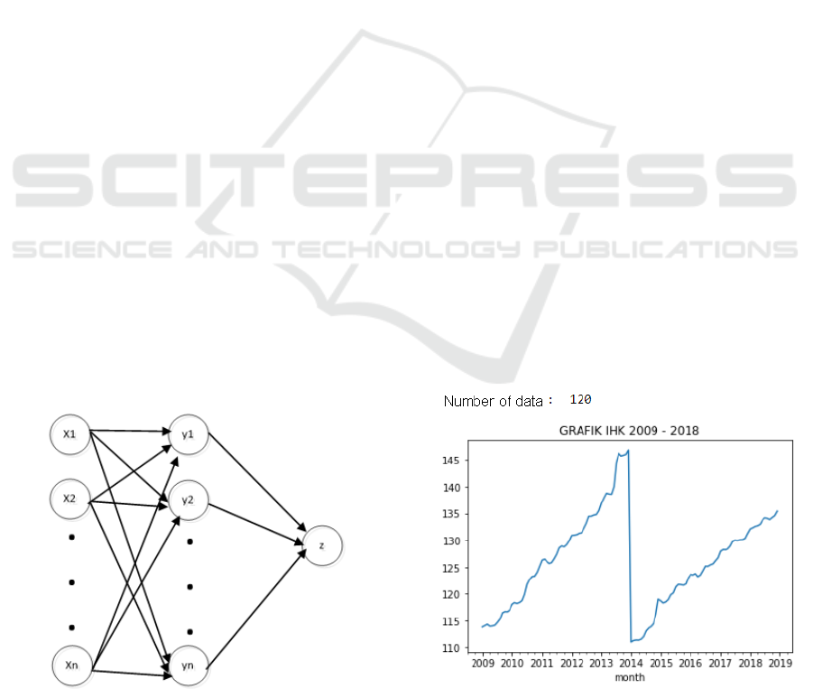
feed-forward section. Figure 1 is the general form of
a traditional ANN, where 𝑥

,𝑥

,…,𝑥

are nodes in
the input layer, 𝑦

,𝑦

,…,𝑦

are nodes in hidden
layers, and 𝑧 is the output layer.
Figure 1: A traditional ANN architecture.
3 RESULTS AND DISCUSSIONS
All methods in this research are implemented in
Python.
3.1 ARIMA Forecasting
3.1.1 Data Identification
The data identification stage is carried out to identify
whether the data to be used met the ARIMA method
requirements' assumptions or not, which is
stationary. If the resulting data is non-stationary, it is
necessary to carry out the differencing stages first.
Based on the plot in Figure 2(a), the time series data
for the CPI value are still non-stationary, with a
trend that tends to be linear starting in 2009. In
2014, the plot showed that the CPI value decreased
drastically with a massive difference in values and
returned to a linear pattern until 2018. Therefore,
data must be processed with the differencing step to
produce stationary data. Figure 2(b) plots the data
after a differencing process of level one.
Because it has passed one differencing level, the
ARIMA model (p, d, q) is now ARIMA (p, 1, q).
Meanwhile, the p and q values can be determined
through the correlation test between the time series
by utilizing the ACF and PACF.
After getting the temporary model ARIMA (p, 1,
q), the next step is to calculate the ACF and PACF
from the data and then plot them. The data used to
calculate ACF and PACF is stationary data, which
come from the first level of differencing. Thus, the
number of data calculated is 108 data, because the
12 initial data in the 2009 period did not have the
results of differencing calculations.
(a)
Time-series Modeling for Consumer Price Index Forecasting using Comparison Analysis of AutoRegressive Integrated Moving Average and
Artificial Neural Network
601

(b)
Figure 2: Plot of CPI Data (a) before and (b) after
differencing step.
3.1.2 Model Parameter Estimation
The data used to calculate ACF and PACF are
stationary (from the first level of differencing).
Thus, the number of data to be calculated is only 108
data because the 12 initial data in the 2009 period
did not have the results of differencing calculations.
In ACF and PACF, there is a lag term used to
determine how many ACF and PACF values will be
calculated. On this 108 CPI data, the number of lags
is n / 4 = 108/4 = 27 lag. Because ACF and PACF
are only used to support transient parameter
estimates and determine p and q models, the
calculations use Python's already available
functions. The ACF and PACF calculations results
are in Figure 3(a) and 3(b), respectively.
In Figure 3(a), the ACF value in lag 1 is outside
the blue line, which indicates that the series still
influence or correlate. The ACF value is used to
estimate the value of the MA or q parameter. Thus,
based on the displayed graph, it can be estimated
that the Indonesian CPI time series model used is a
moving average model. Also, because the graph is
disconnected at lag 1, the provisional model
estimates show that the MA parameter is 1.
The ARIMA pattern (p, 1, q) now becomes
ARIMA (p, 1,1). If the ACF value is used to indicate
the MA parameter, the PACF value indicates the AR
or p parameter. Based on Figure 3(b), because the
blue line also breaks lag one, it can be estimated at
this time, the time series model also contains an
autoregressive pattern. The p parameter has now
also changed its value to 1. Identification for the
estimated parameter ARIMA (p, d, q) is now known;
all the parameters are ARIMA (1,1,1). Furthermore,
the ARIMA model (1,1,1) will be used to formulate
forecasting the value of Indonesia's CPI.
(a)
(b)
Figure 3: ACF (a) and PACF (b) calculations.
3.1.3 ARIMA Forecasting Result
From the estimated ARIMA parameters (p, d, q),
forecasting the CPI value in 2018 will use ARIMA
(1,1,1). The coefficients for AR and MA are
1.309 𝑥 𝑒

and 4.760 𝑥 𝑒

, respectively. The
overall results for the 12 months in 2018 using
ARIMA (1,1,1) are in Figure 4. The Minimum
Square Error (MSE) is also computed.
Figure 4: ARIMA Forecasting and its MSE.
The forecast value generated by ARIMA has a
reasonably large error. However, the ARIMA
forecast value can still be useful if the next stage's
testing is in the CPI value range.
3.2 ANN Forecasting
The training and testing data to be used as input on
ANN need to be normalized first to get values from
CESIT 2020 - International Conference on Culture Heritage, Education, Sustainable Tourism, and Innovation Technologies
602

0 to 1. Normalized training and testing data have
seven columns (including the last column as
CLASS), so the initial ANN architecture is 7-x-1.
The x value is determined by experimenting on
different values such as 8, 9, 10, and 14, and the best
value (which has the lowest MSE of 59.23) is 14.
Therefore, the ANN architecture 7-14-1 is used in
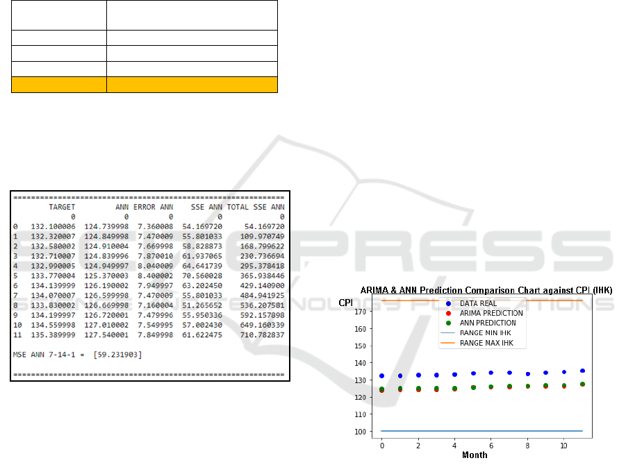
the forecasting phase. Table 1 lists the MSE
comparison of four ANN architectures.
Table 2: MSE Comparison of four ANN architectures.
ANN
Architecture
MSE
Denormalized Output
7
–
8 -1 77.35
7 – 9 – 1 70.26
7
–
10
–
1 65.07
7 – 14 – 1 59.23
3.3 ANN Forecasting Result
The ANN 7-14-1 is used to forecast the CPI value in
2018, and the result is in Figure 5.
Figure 5: ANN Forecasting and its MSE.
The forecast value generated by ANN has a
lower error than ARIMA, which is 59.23.
3.4 CPI Range
The CPI range is calculated based on the price of
goods in the current year used to predict (i.e., 2018)
and the price of goods in the base year. Due to the
large number of types of goods included in each
category, this study only used a sample of 6 prices of
most consumed goods from each category per year.
For the clothing category, the item prices used
are men's t-shirts, women's t-shirts, men's
underwear, women's panties, men's jeans, women's
jeans, sarongs, and Muslim prayer gown (mukena).
For the food category, the prices of goods used are
instant noodles, meatballs, fresh milk, cooking
spices, chicken meat, and cigarettes. For the housing
category, the prices of goods used are house contract
rates, builders' rates, iron blocks, plywood, sand, and
wall paint. As for the health category, the prices of
goods used are general practitioner rates, hospital
rates, drug prices, vitamins, men's haircuts and
women's haircuts. From the calculation, the
estimated CPI range for 2018 is between 100 - 176.
3.5 Comparison Analysis
Figure 6 compares ARIMA and ANN result in
predicting the CPI value for the year 2018. The
lower limit of the CPI range is marked with a
straight blue line that stretches across the value 100
and the upper limit of the CPI range is marked with
an orange straight line that stretches across the value
176. The actual CPI value data obtained from BPS
as a reference for comparison is marked with blue
circles for twelve data (representing each month),
while the ARIMA forecast data is marked with a red
circle. And the ANN forecast data is marked with a
green circle. Both ARIMA and ANN results lie
almost on the same line and are still in the blue-
orange lines' accepted range, representing the min
and max CPI range. Therefore, these two methods
are sufficient enough to forecast the CPI data model.
Figure 6: ARIMA and ANN Result Comparison
4 CONCLUSIONS
This research has resulted in several conclusions as
follows. Firstly, both methods (ARIMA and ANN)
can be used to predict the Indonesian CPI value from
January 2018 - December 2018. The ARIMA model
applied to this forecast is ARIMA (1,1,1) and
produces CPI values of 123.77, 124.08, 124.05,
124.16, 124.66, 125.55, 125.83, 125.75 125.91,
125.93, 126.19, and 127.12. Meanwhile, ANN
Time-series Modeling for Consumer Price Index Forecasting using Comparison Analysis of AutoRegressive Integrated Moving Average and
Artificial Neural Network
603

applies four forms of ANN architectures, which are
ANN 7-8-1, 7-9-1, 7-10-1, and 7-14-1. However, the
best form is 7-14-1 because it produced the smallest
MSE value of 59.23, with the resulting CPI forecast
values of 124.73, 124.84, 124.91, 124.83, 124.94,
125.37, 126.19, 126.59, 126.66, 126.72, 127.01, and
127.54.
Secondly, although both methods can be used for
forecasting, ANN provides better forecasting results
than ARIMA in forecasting research for the
Indonesian CPI value, with a difference of 9.09 in
MSE values, where ARIMA produced an MSE of
68.32 while ANN produced an MSE of 59.23.
However, although the resulting MSE is quite large,
all of the predicted values from these two methods
are still in the CPI range between 100 and 176. So it
can be said that the ARIMA and ANN forecast
results are at a reasonable level and can still be
calculated.
ACKNOWLEDGEMENTS
The authors would like to thank the Faculty of
Computer Science, Universitas Pembangunan
Nasional "Veteran" Jawa Timur, for its support to
publish this research.
REFERENCES
Adebiyi, A. A., Adewumi, A., & Ayo, C. (2014). Stock
price prediction using the ARIMA model. Proceedings
- UKSim-AMSS 16th International Conference on
Computer Modelling and Simulation, UKSim 2014.
doi:10.1109/UKSim.2014.67
Box, G. E., Jenkins, G. M., Reinsel, G. C., & Ljung, G. M.
(2016). Time series analysis : forecasting and control
(5th edition). New Jersey: Wiley.
Deswina, A. P., & Desmita, E. (2015). Application of The
Box-Jenkins Method in Predicting the Consumer Price
Index in Pekanbaru City (Penerapan Metode Box-
Jenkins Dalam Meramalkan Indeks Harga Konsumen
Di Kota Pekanbaru). Jurnal Sains Matematika dan
Statistika, 1(1), 39-47.
Djawoto, D. (2010). Advanced Forecasting of Inflation
with Auto Regressive Integrated Moving Average
(ARIMA) Method (Peramalan Laju Inflasi Dengan
Metode Auto Regressive Integrated Moving Average
(ARIMA)). Jurnal Ekonomi dan Keuangan, 14(4),
524-538.
Domingos S. de O. Santos Júnior, J. F. (2019). An
intelligent hybridization of ARIMA with machine
learning models for time series forecasting.
Knowledge-Based Systems, 175, 72-86.
Fitriani, B. E., Ispriyanti, D., & Prahutama, A. (2015).
Forecasting Loads of Electricity Usage in Central Java
and the Special Region of Yogyakarta Using Hybrid
Autoregressive Integrated Moving Average - Neural
Network (Peramalan Beban Pemakaian Listrik Jawa
Tengah dan Daerah Istimewa Yogyakarta dengan
Menggu). Jurnal Gaussian, 745-754.
Hiteshi Tandon, P. R. (2020). Coronavirus (COVID-19):
ARIMA based time-series analysis to forecast near
future. Cornell University.
Janah, S. N., Sulandari, W., & Wiyono, S. B. (2014).
Application of The ARIMA Backpropagation Hybrid
Model for Price Forecasting of Indonesian Gabah
(Penerapan Model Hybrid Arima Backpropagation
Untuk Peramalan Harga Gabah Indonesia). Media
Statistka, 7(2), 63-69.
Mohamed, J. (2020). Time Series Modeling and
Forecasting of Somaliland Consumer Price Index: A
Comparison of ARIMA and Regression with ARIMA
Errors. American Journal of Theoretical and Applied
Statistics, 9(4), 143-153.
Nopirin. (1987). Monetary Economy (Ekonomi Moneter),
Book II . Yogyakarta: BPFE-UGM.
Pimpi, L. (2013). Implementation of ARIMA Method to
Forecast Indonesia Consumer Price Index (CPI) 2013
(Penerapan Metode ARIMA dalam Meramalkan
Indeks Harga Konsumen (IHK) Indonesia Tahun
2013). Paradigma, 17(2), 35-46.
Susilokarti, D., Arif, S. S., Susanto, S., & Sutiarso, L.
(2015). Comparative Study of Rainfall Prediction Fast
Fourier Transformation (FFT) Method, Autoregressive
Integrated Moving Average (ARIMA) and Artificial
Neural Network (ANN) (Studi Komparasi Prediksi
Curah Hujan Metode Fast Fourier Transformation
(FFT), Autore). agriTECH, 241-247.
Ümit Çavuş Büyükşahin, Ş. E. (2019). Improving
forecasting accuracy of time series data using a new
ARIMA-ANN hybrid method and empirical mode
decomposition. Neurocomputing, 361, 151-163.
doi:https://doi.org/10.1016/j.neucom.2019.05.099
Wigati, Y., Rais, R., & Utami, I. T. (2015). Time Series
Modeling with the ARIMA Process for Prediction of
Consumer Price Index (CPI) In Palu - Central
Sulawesi (Pemodelan Time Series Dengan Proses
Arima Untuk Prediksi Indeks Harga Konsumen (IHK)
Di Palu – Sulawesi Tengah). Jurnal Ilmiah
Matematika dan Terapan, 12(2), 149-159.
CESIT 2020 - International Conference on Culture Heritage, Education, Sustainable Tourism, and Innovation Technologies
604