Debt Ratio, Debt to Equity Ratio, Net Profit Margin

and Return Effects on Stock Price Assets

Dedek Sriulina Sihombing

and Galumbang Hutagalung

Magister of Management, Prima Indonesia University, Jl.Sekip simpang Sikambing, Medan, Indonesia

Keywords: debt ratio, debt to equity ratio, net profit margin and return on assets to stock prices.

Abstrak: The aims of this study are to determine the effect of debt ratio, debt to equity ratio, net profit margin and

return on assets to stock prices. The results of the partial coefficient of debt ratio, debt to equity ratio, net

profit margin, and return on assets on stock prices were 10.27%, -32.7%, 22.27%, and -41%, respectively.

Meanwhile, the coefficient of determination of the debt ratio, debt to equity ratio, net profit margin and

return on assets to stock prices was 60.3%. Simultaneously, the debt ratio, debt to equity ratio, net profit

margin and return on assets have a significant effect on stock prices.

1 INTRODUCTION

In today's economy, competition in the business

world, especially in the consumer goods industry, is

increasingly competitive. Every company is required

to maintain, develop and improve company

standards in order to achieve the company's vision

and mission. The consumer goods industry sector is

one of the sectors that investors are interested in as a

long-term investment. The share price is one of the

indicators of a company's success, which is indicated

by market strength and the occurrence of trading

transactions of the company's shares in the capital

market. The share price reflects the value of a

company. If the company achieves good

performance, the company's shares will be of great

interest to investors.

According to Fahmi (2014), the debt ratio is a

measure of how much a company is financed by

debt. The use of debt that is too high will endanger

the company because it will fall into the category of

extreme leverage, in which the company is trapped

in a high level of debt and it is difficult to release the

debt burden. The importance of financial ratio for

predicting stock price trends was an important,

debatable issue (Lewellen, 2002).

According to Siegel and Shim in (Fahmi, 2015),

the debt to equity ratio is used as a measure in

analyzing financial statements to show the amount

of collateral available to creditors. Debt to Equity

Ratio is a ratio used to assess debt to equity. This

ratio comparases all debt including current money

with all equity, knowing the amount of funds

provided by the creditor and the owner of the

company. This ratio serves to find out any own

capital used as collateral for debt. For creditors the

greater the ratio is the more unprofitable because the

greater the risk borne by failures that may occur in

the company. The bigger the ratio, in contrast to the

low ratio, the higher the level of funding provided

by the owner and the greater the seurity limit for the

borroweer in the event of loss or depreciation of the

value of assets. This ratio also provides general

guidance on the financial viability and risk of the

company. Debt to equity ratio for each company

diffrent, depending on the business characteristics

and diversity of cash. Companies with stable cash

flow usually have a higher ratio than the less stable

cash ratio (Hapsoro and Husain, 2019)

According to Wahyudiono (2014), when a

company has a high profit margin, it usually has a

better competitive advantage. Companies with high

net profit margins will automatically have the ability

to protect themselves during difficult times. On the

other hand, companies with low margins tend to

keep going down. Profit margin with competitive

profit level will be able to help the company and

have a market niche even in difficult times. Net

profit margin measures how much profit out of each

sales dollar is left after all expenses are subtracted

that is, after all operating expenses, interest, and

income tax are subtracted (Andrews,2007)

530

Sihombing, D. and Hutagalung, G.

Debt Ratio, Debt to Equity Ratio, Net Proﬁt Margin and Return Effects on Stock Price Assets.

DOI: 10.5220/0010335600003051

In Proceedings of the International Conference on Culture Heritage, Education, Sustainable Tourism, and Innovation Technologies (CESIT 2020), pages 530-535

ISBN: 978-989-758-501-2

According to Pandia (2012), a bank must have

the ability to measure management's ability to gain

overall benefits. The greater the ROA of a bank, the

greater the level of profit and the better the position

of the bank in terms of asset use. High return on

assets indicates how well the assets are managed by

the companies to bring profit for each one dollar of

asset that has been invested to the company (Gut et

al.2011). Return on assets is one of profitability

ratios. In the analysis of financial statements, this

ratio is most often highlighted, because it is able to

indicate company succes to create profits. ROA is

able to measure the company ability to generate

profits in the past to then be projected in the future.

2 RESEARCH METHODS

In this research, the method used is quantitative

(Sugiyono 2013) with descriptive statistics. The

sampling technique used was purposive sampling.

The population seen in the study is 37 consumer

goods industry companies listed on the Indonesia

Stock Exchange for the period 2012-2017. Types

and sources of data used come from secondary

sources.

According to Sugiyono (2013), secondary data

sources are data sources that are not directly

processed by data collectors, for example through

other people or through documents. Secondary data

used comes from financial reports, journals or

company annual reports obtained from

www.idx.co.id.

3 RESEARCH RESULTS AND

DISCUSSION

3.1 Descriptive Statisctics

Based on the result of the analysis of statistical

description, it follows in table 1 shown the

characteristics of the sample used in this study

include: number of samples (N), sample mean,

maximum value for each variable

Table 1: Descriptive Statistic Test.

Variabel N Minimu

Maximu

Mean

DR 90 ,07132 ,75178 ,3676046

DER 90 ,15018 171,40450 3,5477355

NPM 90 ,01982 ,39002 ,1199222

ROA 90 ,02969 ,65720 ,1525569

Stock Prie 90 180 1200000 47546,44

Valid N 90

Sources: Processed Secondary data.

Table 1 above shows that the number of observation

in the Consumer Goods in Indonesia stock exchange

2012-2017 period in this study is 90 sample. The

lowest(minimum) of stock price is 180 and the

highest (maximum) of stock price is 120000000.

Variabel Debt ratio has the smallest value

(minimum) of 0,07132 and the largest

(maximum)0,75178.

3.2 Normality Test

Normality test aims to obtain a regression model and

confounding or residual variables. The normality test

is used to test whether the data is normally

distributed or not. The following is a test of the

results of data normality in the form of a histogram

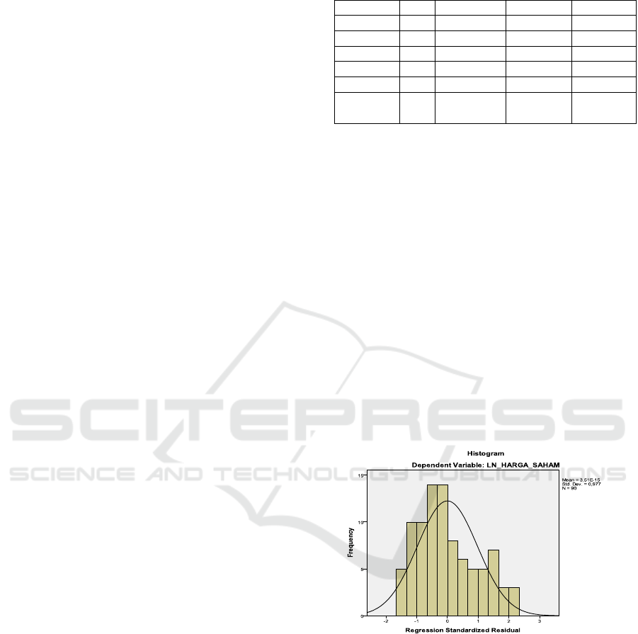
graphic in Figure 1.

Figure 1: Normality Test.

Sources: Processed Secondary data.

Based on Figure 1 Graphical display is data that has

normal distribution. The histogram graph shows that

the data is symmetrical or not tilted to the right and

left.

Normality test data statistical analysis can be

done using Kolmogorov – smirrnov. In multivariate

data normality test performed on residual value .

The data indicated normal distribution with

significant value above 0,05(Ghozali,2006). The

data shown in table 2 below:

Debt Ratio, Debt to Equity Ratio, Net Proﬁt Margin and Return Effects on Stock Price Assets

531

Table 2: On-Sample Kolmogorov Smirnov Test.

Untandardized

Residual

N 90

Normal Parameters

Mean

,0000000

Std. Deviation 1,45403293

Most Exxtreme

Differences Absolute

,105

Positive ,105

Negative -,075

Kolmogorov – Smirnovz ,991

Asymp. Sig(2-tailed) ,279

Based on the result in table 2 above, from the result

of the second test, it shows that the data was

normally distributed. This is indicated by the test

Kolmogorov – smirrnov showed result that

significance level of 0,279 which is far above 0,05.

3.3 Multicolinearity Test

Multicolinearity test aims to test whether the

regression model shows a correlation relationship

between independent variables (independent). A

good regression model should not have a correlation

between the independent variables. If the

independent variables correlate with each other, then

the independent variable which has a correlation

value between independent variables is equal to

zero. To determine the absence of multicolinearity, it

can be seen from the Variance Inflation Factor (VIF)

value and the Tolerance value. With the criteria, if

the Variance Inflation Factor (VIF) value is <0.10

then there is no multicollinearity, but if the VIF

value> 10 then there is multicollinearity. Tolerance>

0.1 means there is no multicollinearity and vice

versa.

Table 3: Multicolinearity Test.

Variables Tolerance VIF

Debt Ratio 0,747 1,338

Debt to Equity 0,810 1,234

Net Profit Margin 0,189 5,285

Return On Asset 0,209 4,774

Sources: Processed Secondary data.

Based on Table 3, the following conclusions can be

drawn: (i) debt ratio with a tolerance value of 0.747

greater than 0.10 and a VIF value of 1,338 less than

10. (ii) debt to equity ratio with a tolerance value of

0.810 greater than 0.10 and a VIF value of 1,234 less

than 10. (iii) net profit margin with a tolerance value

of 0.189 greater than 0.10 and a VIF value of 5,285

less than 10. (iv) return on assets with a tolerance

value of 0.209 greater than 0.10 and a VIF value of

4,774 less than 10. (v) Because the tolerance value

obtained by each variable is greater of 0.10 and the

VIF value obtained for each variable is less than 10,

the data for the variable debt ratio, debt to equity

ratio, net profit margin and return on asset do not

have multicollinearity.

3.4 Autocorrelation Test

The autocorrelation test aims to see whether in a

linear model there is a correlation between

confounding errors in period t with errors in period

t-1 (previous). This value is used as a measure in

determining the presence or absence of an

autocorrelation problem.

Table 4: Durbin watson.

Durbin Watson

2,135

Sources: Processed Secondary data.

The results on table 4 the Durbin-Watson

statistical value (d) = 2.135 and du = 1.7508,

namely: 0 <1.7508 <2.135 <2.2492. DW value 2.135

which is greater than du 1.7508 and less than 4 -

1.7508 = 2.2492, it can be concluded that the Durbin

Watson test does not have autocorrelation.

3.5 Coefficient of Determination(R

)

The coeffiient od determination (R

) essentially

measures how far the ability of the model to explain

variations in the dependent variable. R

value close

to one means independent variables provit almost

all the information needed to predict the variation of

thw dependent variable (Ghozali,2006). The

determination coefficient calculation result can

beseen in Table 5 bellow :

CESIT 2020 - International Conference on Culture Heritage, Education, Sustainable Tourism, and Innovation Technologies

532

Table 5: Determination Coeefficiebt (R

R R square Adjusted R

square

Std.Error of

the Estimate

Durbin

Watson

,603 ,364 ,334 1,48785 2,135

Sources : Processed Secondary data

The value of R square is 0.364, it mean 36.4%

stock price variation can be explained by the

variation of independent variable which are debt

ratio, debt to equity ratio, net profit margin, and

return on asset. On the other hand the rest of

percentage whichis 63,6% will be explained by other

variables outside the model research.

4 ANALYSIS RESULT

Analysis of the data used in this study is based on

multiple linear regression equations to find the

relationship or influence between the independent

variable on the dependent variable Stock Price. The

following are the results of multiple linear regression

analysis which can be seen in Table 6.

Table 6: Multiple linear regression.

Variable Unstandardized

Coefficients

T Sig

B Std.Error

(Constant) 14,009 ,883 15,862 ,000

Debt ratio 1,027 ,399 2,576 ,012

Debt to

Equity Ratio

-,327 ,169 -1,936 ,056

Net Profit

Margin

2,227 ,558 3,992 ,000

Return On

Asset

-,410 ,508 -,806 ,442

Sources : Processed Secondary data.

The result on Table 6 multiple linear regression

equation as follow:

LN_HARGA SAHAM = 14,009 + 1,027 Debt Ratio

– 0,327 Debt to Equity Ratio + 2,227 Net Profit

Margin – 0,410 Return On Asset

The regression equation above has the following

meanings: (i) The debt ratio regression coefficient of

was 1.027(ii) The debt to equity ratio regression

coefficient of was -0,327 (iii) The net profit margin

regression coefficient of was 2,227 (iv) The return

on asset regression coefficient of was -0,410. (v)

The constant value of 14,009 shows that if the

variable value of Debt ratio, Debt to Equity Ratio,

Net Profit Margin and Return On Asset is

considered constant, then the value of the Share

Price (Y).

4.1 Effect of Debt Ratio on Stock Prices

The hypothesis to be tested states that there is an

effect of debt ratio on Stock Prices.

Tabel 7: debt ratio on stock prices.

Variabel

Independen

Koefisien

Standar

Error

T Signifikan

Debt Ratio 0,258 2,57

0,012

R= 0,33

= 0,001

Estimasi Standar Error = 0,399

F= 12,172

Variabel dependen Stock Price

Sources : Processed Secondary data

From the test results in Table 7, it is found that the

results of the debt ratio test on stock prices have a

positive and significant effect with the value of F =

12.172 at p <0.012 (strong relationship). This can be

seen from the magnitude of R = 0.33, the R

value of

0.001, and the Estimated Standard Error of 0.399.

The partial debit ratio has a t-

count

value of 2.576 and

a t-

table

value at the confidence level of 95%

(significant 5% or 0.005) with a degree of freedom

(df) of 1.99394 so that tcount = 2.576> ttable =

1.98793 and a significant value of 0.012 <0 , 05.

These results indicate that HO is rejected and Ha is

accepted, which means that partially the debt ratio

has a significant effect on stock prices.

4.2 Effect of Debt to Equity Ratio on

Stock Prices

The hypothesis to be tested states that there is an

effect of debt to equity ratio on stock prices.

Debt Ratio, Debt to Equity Ratio, Net Proﬁt Margin and Return Effects on Stock Price Assets

533

Table 8: Debt to equity ratio on stock prices.

Variabel

Independen

Koefisien

Standar

Error

t Signifik

Debt to

equity ratio

1,83252 -1,936 0,056

R= 0,38

= 0,001

Estimasi Standar Error = -0,186

F= 12,172

Variabel dependen Stock Price

Sources: Processed Secondary data

From the test results in Table 8 it is found that

the test results of the debt to equity ratio on stock

prices have no effect and are significantly positive

with a value of F = 12.172 at p <0.056 (weak

relationship). This can also be seen from the

magnitude of R = 0.38, the value of R

= 0.001, and

the standard error estimate of -0.186. The Debt to

Equity Ratio partially has a t-

count

value of -1.936

and a t-

table

value of 1.98793 so that t

count

table

with a

significant value of 0.056> 0.05. These results

indicate that Ha is rejected and Ho is accepted,

which means that partially the Debt to Equity Ratio

has no effect on stock prices.

4.3 Effect of Net Profit Margin on

Stock Prices

The hypothesis to be tested states that there is an effect of

net profit margin on stock prices

Table 9: Net Profit Margin on stock prices.

Variabel

Independen

Koefisien

Standar

Error

t Signifik

Net Profit

Margin

0,794 3,992 0,000

R= 0,553

= 0,306

Estimasi Standar Error = 0,558

F = 12,172 pada p < 0,000

Variabel dependen Stock Price

Sources: Processed Secondary data.

From the test results in Table 9 it is found that the

test results of the net profit margin on stock prices

have a positive and significant effect with the value

of F = 12.172 at p <0.000 (strong relationship). This

can be seen from the magnitude of R = 0.553, the

value of R

= 0.306, and the Estimated Standard

error of 0.558. Partially, Net Profit Margin has a t-

count

value of 3.992 and a t-

table

value of 1.98793 so

that t

count

> t

table

with a significant value of 0.000

<0.05. These results indicate that Ha is rejected and

Ho is accepted, which means that partially the Net

Profit Margin affects the stock price.

4.4 Effect of Return on Assets on Stock

Prices

The hypothesis to be tested states that there is an effect of

return on asset on stock prices

Table 10: return on asset on stock prices.

Variabel

Independen

Koefisien

Standar

Error

T Signifikan

Return on asset -0,152 -0,806 0,422

R= 0,482

= 0,233

Estimasi Standar Error = 0,169

F = 12,172 pada p < 0,508

Variabel dependen: Stock Price

Sources : Processed Secondary data.

From the test results in table 10, it is found that the

test results of the net profit margin on stock prices

have a positive and significant effect with the value

of F = 12.172 at p <0.000 (strong relationship). This

can be seen from the magnitude of R = 0.553, the

value of R

= 0.306, and the Estimated Standard

error of 0.558. Partially, Net Profit Margin has a t-

count

value of 3.992 and a t-

table

value of 1.98793 so

that t

count

> t

table

with a significant value of 0.000

<0.05. These results indicate that Ha is rejected and

Ho is accepted, which means that partially the Net

Profit Margin affects the stock price.

4.5 Simultaneous Test Result (Test F)

Simultaneous hypothesis testing or the F test is

carried out to test how the influence between

independent variables together on the dependent or

dependent variable

CESIT 2020 - International Conference on Culture Heritage, Education, Sustainable Tourism, and Innovation Technologies

534

Table 11: Test F.

Variabel

Independen

Estimasi

Standar

Error

F Signifik

Regression_R

esidual

1,48785 12,172 0,000

R= 0,603

= 0,364

Estimasi Standar Error = 1,48785

F = 12,172 pada p < 0,000

Predictors : (Constant) Debt ratio, debt to equity ratio ,

net profit margin, return on assets

Dependent Variable: Stock Price

Sources : Processed Secondary data.

From the test results in table 10, It was found that

the value of F

count

was 12,172> F

table

value, namely

df = (n-k-1) = 2.48 with a significant value of 0.000

<0.05. This can be seen from the magnitude of R =

0.603 and the Estimated Standard error of 1.48785.

From these results it can be concluded that Ho is

rejected and Ha is accepted, meaning that together

all independent variables consisting of debt to asset

ratio, debt to equity ratio, net profit margin and

return on assets simultaneously have a significant

effect on stock prices.

5 CONCLUSIONS

Based on the results of research in the previous

chapter, the conclusions that can be obtained from

this study are: (i) Partially debt ratio and Net Profit

Margin have a significant positive effect on prices

(ii) Debt to Equity Ratio and Return on Assets

partially have no significant positive effect to stock

prices, (iii) Debt to Equity Ratio, Net Profit Margin,

Return On Asset simultaneously have a significant

effect on stock prices in Goods Industrial Companies.

REFERENCES

Andrew, Joseph D., 2007. Financial Management:

Principle and Practice, Freeload Press. United State, 4

Edition.

Brigham. Houston., 2010. Dasar-dasar manajemen

keuangan perusahaan, Erlangga. Jakarta, Ed.11

Darmadji, Tjiptono dan Hendry M. Fakhruddin., 2012.

Pasar Modal Indonesia, Salemba Empat. Jakarta.

Fahmi Irham., 2013. Pengantar Pasar Modal, Alfabeta.

Bandung. Cetakan Kedua.

Ghozali, Imam., 2016. Aplikasi Analisis Multivariate

Dengan Program IBM SPSS 21, Badan Penerbit

Universitas Diponegoro. Semarang. Cetakan VII.

Gul S., Irshad, F. & Zaman,K., 2011. Factors Affecting

Bank Profitability in Pakistan, The Romanian

Economic Journal, 14(39), 61-87.

Hanafi, Mamduh., 2014. Analisis Laporan Keuangan. Edisi

Keempat, Sekolah Tinggi Ilmu Manajemen YKPN.

Yogyakarta.

Hapsoro, D., & Husain, Z.F., 2019. Does Sustainability

report moderate the effect of financial performance on

Investor reaction. Evidence of Indonesian listed firms.

International Journal of Business.

Hery., 2011. Akuntansi: Aktiva, Utang Dan Modal, Gava.

Yoyakarta. Cetakan Kesatu.

Horne, James C. Van dan Jhon., 2012. Prinsip-prinsip

manajemen keuangan. Salemba Empat. Jakarta. Edisi

13.

Lewellen, J., 2002. Predicting Return With Financial

Ratios. MIT Sloan School of Management : Working

Paper

Prastowo., 2014. Analisis Laporan Keuangan: Konsep dan

Aplikasi, Sekolah Tinggi Ilmu Manajemen YKPN.

Yogyakarta, Cetakan Kedua.: Ed 3.

Riyanto, Bambang., 2010. Dasar - Dasar Pembelanjaan

Perusahaan, BPFE. Yogyakarta, Cetakan Kedua Belas.

Rodoni, Ali., 2014. Manajemen Keuangan Modern, Mitra

Wacana Media. Jakarta.

Sartono, Agus., 2012. Manajemen Keuangan Teori dan

Aplikasi, BPFE. Yogyakarta, Edisi Keempat.

Sugiyono., 2013. Metode Penelitian Kuantitatif Kualitatatif

dan R&D, Alfabeta. Bandung, Edisi Baru.

Sunyoto, Danang and Fathonah Eka Susanti., 2015.

Manajemen Keuangan Untuk Perusahaan: Konsep dan

Aplikasi, CAPS. Yogyakarta, Cet.1.

Debt Ratio, Debt to Equity Ratio, Net Proﬁt Margin and Return Effects on Stock Price Assets

535