Detection of Objects and Trajectories in Real-time using Deep Learning

by a Controlled Robot

Adil Sarsenov, Aigerim Yessenbayeva

, Almas Shintemirov

and Adnan Yazici

Department of Computer Science, Nazarbayev University, 53 Kabanbay Batyr Ave, Nur-Sultan, Kazakhstan

Keywords:

Deep Learning, Object Detection, Trajectory, Depth Camera, LIDAR.

Abstract:

Nowadays, there are many different approaches to detect objects as well as to determine the trajectory of an

object. Each of these approaches has its advantages and disadvantages in terms of real-time use for various

applications. In this study, we propose an approach to detect objects in real-time using the YOLOv3 deep

learning algorithm and plot the trajectory of an object using 2D LIDAR and depth cameras on a robot. The

laser rangeﬁnder allows us to ﬁnd distances to objects from a certain angle, but does not provide accurate

object detection of the object class. In order to detect the object in real-time and discover the class to which

the object belongs, we formed YOLOv3 deep learning model using transfer learning on several classes from

data sets of publicly accessible images. We also measured the distance to an object using a depth camera with

LIDAR together to determine and estimate the trajectory of objects. In addition, these detected trajectories are

smoothed by polynomial regression. Our experiments in a laboratory environment show that YOLOv3 with

2D LIDAR and depth camera on a controlled robot can be used fairly accurately and efﬁciently in real-time

situations for the detection of objects and trajectories necessary for various applications.

1 INTRODUCTION

In recent years, the robotization of all spheres of hu-

man activity is gaining momentum. A technologi-

cal breakthrough in robotics and machine learning al-

lows people to build autonomous vehicles and various

robots to work autonomously. Mobile robots typically

focus on solving a wide range of diverse applications

to collect heterogeneous information and to be able to

perform technological operations in extreme environ-

ments. Almost every robot needs input sensors like

a laser scanner (LIDAR) or a camera to perceive the

environment that surrounds it. LIDAR is a device that

measures distances to targets at speciﬁc angles and is

used for light detection and ranging. The rapid evo-

lution of the technological level tends to lower the

prices of the various sensors including the 2D and 3D

LIDARs. 2D LIDAR can only estimate the distance

to objects. For this reason, the data that can be ex-

tracted from LIDAR is the only array of ranges to the

objects.

https://orcid.org/0000-0002-0128-3634

https://orcid.org/0000-0002-6969-8529

https://orcid.org/0000-0001-9404-9494

The main objective of this study is to recognize

the object in the image frame and to estimate its po-

sition to trace the trajectory of the object, which is

supplemented by the use of the Jaguar mobile robot.

The robot is equipped with 2D Hokuyo LIDAR, an IP

camera, a depth camera and a Raspberry Pi, which are

the main components of our system architecture. The

Raspberry Pi will serve as a processor and data trans-

mitter, whose data collected from LIDAR and cam-

eras are sent to the PC via Wi-Fi for further process-

ing (Lu, 2018). In this study, we propose the use of a

deep learning algorithm on LIDAR data to detect the

bounding boxes in the images to increase awareness

around the environment and the use of the distance to

a speciﬁc angle of the object obtained from LIDAR

which can help locate an object and retrace its trajec-

tory. The distances and angles returned by LIDAR

are used with a distance to an object using the depth

camera to construct the trajectory of an object.

Object detection is performed using the You Look

Only Once v3 (YOLOv3) algorithm. In order to re-

duce the size of the training data, the transfer learning

approach with pre-trained weights is applied. The ﬁ-

nal step is to locate the object by returning its Carte-

sian coordinates and plotting the trajectory path. The

source of a dataset is images (Kuznetsova and at. al.,

Sarsenov, A., Yessenbayeva, A., Shintemirov, A. and Yazici, A.

Detection of Objects and Trajectories in Real-time using Deep Learning by a Controlled Robot.

DOI: 10.5220/0010215201310140

In Proceedings of the International Conference on Robotics, Computer Vision and Intelligent Systems (ROBOVIS 2020), pages 131-140

ISBN: 978-989-758-479-4

131

2018) for our deep learning algorithm for the detec-

tion of objects requiring big data. The transfer learn-

ing (Tan and at. al., 2018) is a technique that avoids

training the model from scratch by training your own

rather smaller data size using pre-trained weights. It

therefore applies the previous knowledge acquired by

the huge amount of data to new small data speciﬁc to

an application.

The main contributions of the study are as follows.

• We propose accurate and robust solutions for

the detection and localization of objects in real

time on a system architecture composed of a 2D

Hokuyo LIDAR, an IP camera, a depth camera

and Raspberry Pi. In addition, we have tested and

validated this proposed architecture in a labora-

tory environment on a robot equipped with these

components.

• We train YOLOv3 deep learning algorithm on

open-source datasets and use obtained parameters

for real-time object detection instead of using tra-

ditional object detection approaches, which are

relatively slow.

• 2D Hokuyo LIDAR is used to ﬁnd the coordinates

of the object and follow the movement of the de-

tected object. We use polynomial regression on

these generated coordinates to ﬁnd the line that

best ﬁts and smooths the trajectory.

• In addition, the distances measured from the depth

camera are used with the LIDAR angles for the

trajectory plot for an accurate estimation of the

trajectory.

• With our experiments we show that YOLOv3 with

2D LIDAR and depth cameras on a controlled

robot is used fairly precisely in real-time situa-

tions for the detection of objects and the estima-

tion of trajectories necessary for various applica-

tions.

The rest of the article is organized as follows. The

second section includes related work. Section 3

brieﬂy explains the hardware conﬁguration. The

fourth section describes the deep learning algorithm

used for object detection. Section 5 presents trajec-

tory estimation including localization techniques for

measuring distances to objects. The experimental re-

sults are presented and discussed in Section 6. Finally,

we give the conclusion and future work.

2 RELATED WORK

This section provides a review of the literature re-

lated to our study. Viola Jones et al (Wang, 2014)

proposed initial attempts to detect objects on the im-

ages using the features of Haar wavelet and Adaboost

cascading algorithm. Later in 2005, Dalal and Triggs

(Dalal and Triggs, 2005) proposed Histograms of Ori-

ented Gradients (HOG), the HOG feature was more

discriminative than Haar-cascade features. As already

mentioned, deep learning algorithms for the localiza-

tion and detection of objects as well as the use of

these algorithms in the ﬁeld of robotics are the sub-

ject of active research. With the increasing popularity

of deep learning models, HOG functionality has been

replaced by models of convolutional neural networks

(CNN). Nowadays, there are several states of algo-

rithms for the detection and localization of objects in

images. Some examples are the Single Shot MultiBox

Detector (SSD) method (Liu and at. al., 2016), Faster

RCNN (Ren and at. al., 2015), YOLOv3 (Redmon

and Farhadi, 2018), etc.

For real-life applications, there is no straightfor-

ward answer to the question of which of them is the

best. The following sources of literature are more re-

lated to applications that involve object detection in

combination with the various sensors. (Wei and at.

al., 2018) proposes the LIDAR camera and data fu-

sion using fuzzy logic for beacon detection as part of

the multi-sensor collision avoiding system. The study

places LIDAR vertically in order to extract points cor-

related to the beacon from different angles and ap-

plied support vector machines in order to extract char-

acteristics which are later combined with object de-

tection using fuzzy logic. Insu Kim and Kin Choong

Yow in (Kim and Yow, 2015) propose an estimate of

the location of objects from a single camera. They

use HOG to detect an object and estimate the distance

to that object using stereo vision. The state-of-the-art

deep learning classiﬁcation algorithms are provided

in (Ciaparrone and at. al., 2020).

The study in (Krizhevsky et al., 2012) introduces

AlexNet that contains eight layers, ﬁve convolutional

and three fully-connected layers and as an activa-

tion function it uses ReLU. After the success of

the ResNet model (He and at. al., 2015), in 2016

the Inception-v4 and InceptionRes were introduced

(Szegedy and at. al., 2016). The main idea of SENet

(Hu and at. al., 2017) is to learn a weight tensor that

provides different weights for feature maps for each

channel (activation).

3 HARDWARE CONFIGURATION

In this section, we present the preliminary hardware

conﬁguration, including the fundamental context of

the mobile robot, the sensors, the IP camera, the depth

ROBOVIS 2020 - International Conference on Robotics, Computer Vision and Intelligent Systems

132

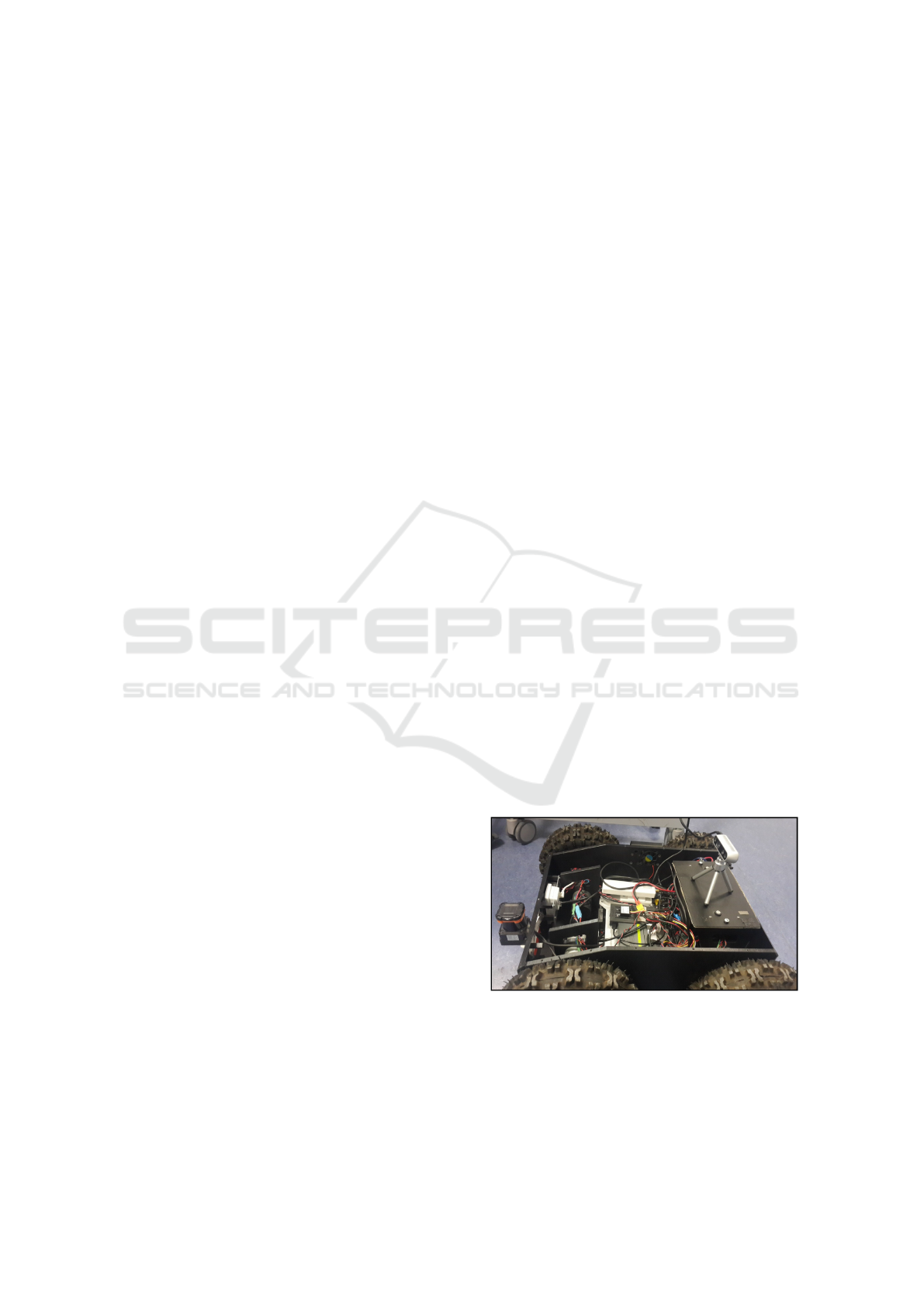
cameras and the Raspberry Pi 3.

The design of a mobile robot is often completely

determined by the environment in which it is used

and based on various parameters (Rincon and at.

al., 2019). In our study, we focus on the Jaguar

4x4 wheeled mobile robotic platform. This robot is

mainly designed for indoor and outdoor navigation.

One of the advantages of this mobile platform is that

it has faster maneuverability and movement capacity

on a vertical stage with a maximum step of 155 mm

and a variety of speed between 0 and 14 km/h.

Sensors are used to convert a certain physical

quantity into an electrical signal. The main task of any

sensor is to respond to external inﬂuences and provide

the system with data on changes in the environment.

There are different types of sensors used in the hard-

ware conﬁguration of our testbed. In particular, for

this study, the sensors detect movement and measure

the distance to objects.

An IP camera is a digital video camera and the

transmission of a video stream through it is done in

digital format on an Ethernet and TokenRing net-

work using the IP protocol (Cabasso, 2009). Spe-

cialized IP cameras often transmit video in an un-

compressed form. IP cameras are often powered by

Power over Ethernet (PoE). Higher resolutions, in-

cluding megapixels, can be used in IP cameras, as

there is no need to transmit an analog signal in Phase

Alternating Line (PAL) or National Television Stan-

dards Committee (NTSC) format. The typical resolu-

tion for network cameras is 650 × 840 pixels. Gener-

ally, IP cameras can be classiﬁed as webcams.

Intel RealSense Depth cameras shoot video, but

in each pixel instead of brightness, there is a point of

depth for each corresponding pixel. These cameras

have been gradually increasing the resolution, depth

accuracy and stability of the output signal, but they

are still relatively imperfect. In our study, we use the

Intel RealSense D435 depth camera (Keselman and

at. al., 2017). The camera has the highest possi-

ble viewing angle and it minimizes the risk of blind

spots appearing and is equipped with a shared shutter,

which guarantees the highest quality and clear percep-

tion of data. The camera has a set of video sensors that

can identify differences in images with resolutions up

to 1280 x 720 pixels. One advantage of the RealSense

camera that comes with its own Intel-supported SDK.

The main objective of RealSense technology is to en-

able a new type of communication and to give the pos-

sibility of interacting with the outside world.

The Raspberry Pi 3 is a single board computer

launched in industrial production in 2012. Initially,

it was intended as an affordable solution to introduce

the basics of programming and global high technol-

ogy. It contains the ARM processor, RAM chips, a

slot for a micro-SD card, as well as an Ethernet port,

HDMI, a 3.5 mm audio output and USB ports for con-

necting peripherals. The majority of the components

required for our mission are already integrated into

the Jaguar mobile platform. It is a good choice for

small storage and data transmission. Due to the ab-

sence of LIDAR among the components of the Jaguar,

we were able to manually mount the LIDAR on top

of the robot hood. The main disadvantage of such a

LIDAR location from the point of view of the build-

ing map and obstacle avoidance is that it does not see

certain objects located below the LIDAR. Other com-

ponents such as the Wi-Fi router and the integrated IP

camera are included in the components of the mobile

platform. Finally, the version fully connected to the

robot’s sensors is visible in Figure 1. We connect the

Raspberry Pi which is inside the Jaguar robot to the

source 5V. In addition, we also connect the LIDAR to

another source 5V and connect it to the Raspberry Pi.

We have made the appropriate conﬁguration and con-

ﬁgured the IP addresses and masks of the global sys-

tem. This conﬁguration is required so that the Rasp-

berry Pi can transmit data from LIDAR directly to the

PC via Wi-Fi. The main computer which acts as a

server receives and then processes the data obtained

from the client which, in our case, is Raspberry Pi.

This simple client-server architectural model allows

data to be processed and transmitted over the network.

The data received from LIDAR is in the form of

an array. The size of each array is 1080 points. The

points represent the distance to each object within the

angle step of the LIDAR. The video stream from the

IP camera is also sent via Wi-Fi. It is possible to sim-

ply connect to the camera via its IP address. The

video frame can be adjusted to the speciﬁc size, the

default is 680 x 480 pixels.

Figure 1: The hardware setup.

4 OBJECT DETECTION

The main objective of object detection is to ﬁnd ob-

jects: pedestrians, bicycles, buildings or any other

Detection of Objects and Trajectories in Real-time using Deep Learning by a Controlled Robot

133

class on images and videos and to annotate them with

the bounding box (Khalifa et al., 2020). In other

words, the output of the object detection is (x, y,

width, height) from the bounding box that contains

the object. On the other hand, object classiﬁcation or

recognition indicates what the object is in the bound-

ing box. Thus, the output of the classiﬁcation is a

class label of the particular bounding box. We use the

YOLOv3 deep learning model for object detection.

Generally, algorithms related to object detection and

its localization within an image consist of two groups:

1. Algorithms built on the classiﬁcation.

2. Algorithms built on the regression.

The algorithms consist of two phases. First, the algo-

rithm selects distinct regions of an image. In addition,

these regions are classiﬁed using CNNs. Prediction is

made for each region selected. Since the algorithm

runs for each selected region, it can be very slow.

The region-based CNN (RCNN) and its modiﬁcations

(Faster-RCNN) are considered as this type of algo-

rithms (Girshick et al., 2013),(Yang and at. al., 2020).

The algorithms based on the second type do not se-

lect the regions offered in an image. Instead, it in-

volves predicting bounding boxes and related classes

in a single execution of the algorithm for the entire

image. The YOLO algorithm belongs to the second

category.

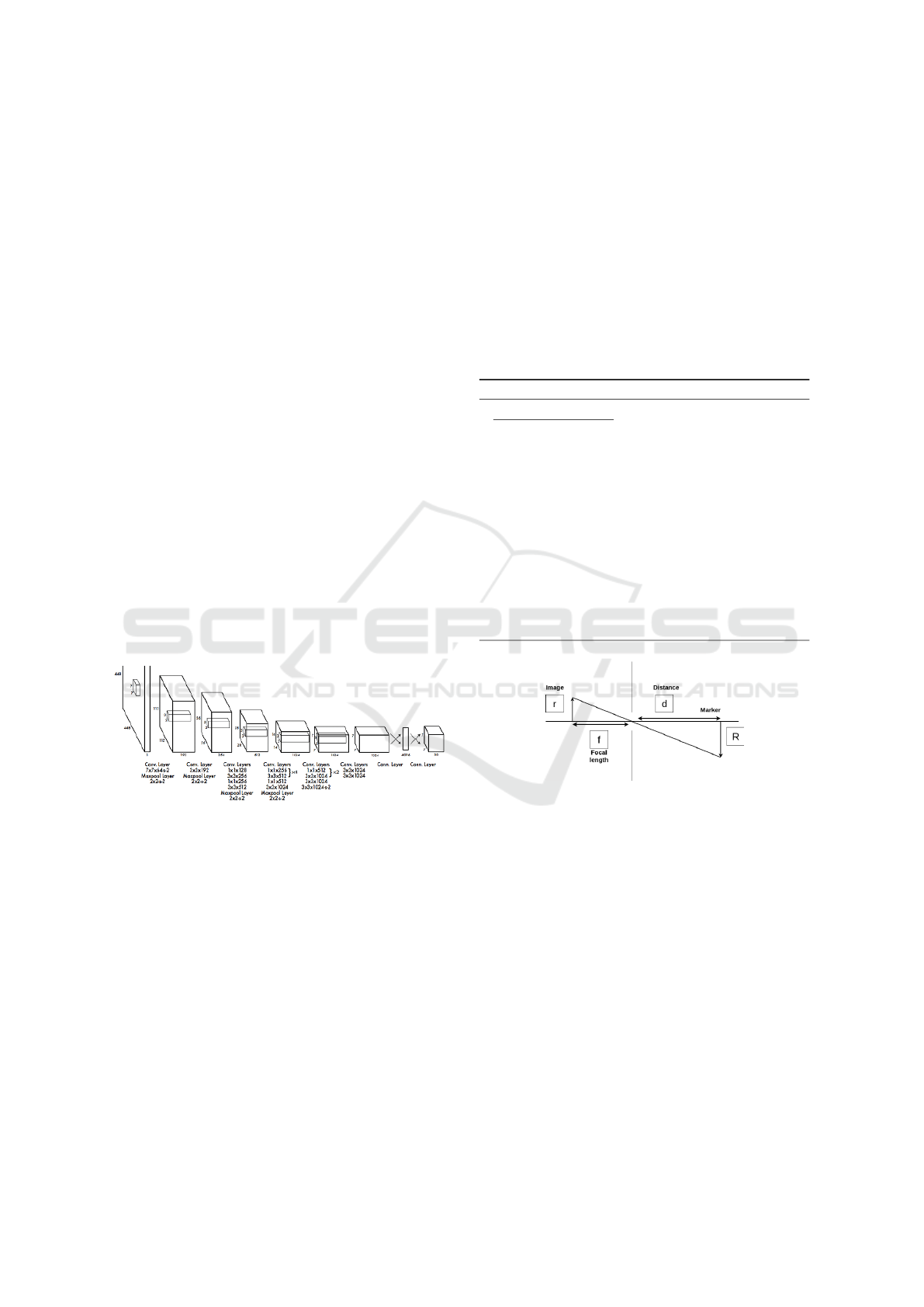
Figure 2: Architecture of CNN (Li and at. al., 2018).

The YOLO algorithm was introduced at the end of

2015 (Redmon and at. al., 2016). YOLO allows fast

image processing compared to CNN, but with lower

accuracy. As mentioned earlier, the YOLO solves the

problem of object detection as a regression problem

and due to the high-speed image processing, it is suit-

able for use in real-time systems.

The CNN model takes the entire image as input

and gives the coordinates of the bounding boxes and

the probability of belonging to classes. The CNN ar-

chitecture is shown in Figure 2. The output of the

CNN is a tensor with coded predictions, and its size

is S × S (B × 5 + C). Here, S denotes the dimen-

sion of a grid and B denotes the number of bounding

boxes. The value C is the number of classes that a NN

is able to recognize.

The YOLOv3 algorithm in terms of mean average

precision (mAP) is superior to the Single Shot Multi-

Box Detector (SSD) method (Liu and at. al., 2016),

but inferior to the Faster R-CNN method (Ren and at.

al., 2015). However, the Faster R-CNN frame does

not process more than 5 frames per second. Using

the NVIDIA Titan X graphics processing unit, the

YOLOv3 algorithm processes images at 30 frames

per second, good for real-time video processing sys-

tems. Therefore, we have chosen the YOLOv3 model

for this study. The pseudo code of object detection

using YOLOv3 is given in Algorithm 1.

Algorithm 1: Real–time Obj. Detection With YOLOv3.

function detectObject (V, t

);

Input: V : video stream

: threshold

Output: Object market with bounding box

for each frame f in V do

//resize frame

f = f.size(416, 416)

//detect objects in frame above threshold

detections = detect (f, td = 0.5)

//draw bounding boxes on detected objects

image = drawBoundingBox(detec–s, frame)

//display image

show(image)

end

return image

Figure 3: Triangle similarity principle.

5 TRAJECTORY ESTIMATION

This section presents the methods of distance and

trajectory measurement. Estimating the distance be-

tween a camera and an object is often offered as an

inexpensive solution to alternative methods such as

the use of laser scanners or radars. In general, there

are several basic methods for estimating the distance

between a particular object and a simple monocular

camera (Kim and Yow, 2015).

We determine the distance to an object using in-

formation about its size. If the real dimensions of an

object (height or width) are known, then, knowing the

coordinates of an object in the image, using the for-

mulas of projective geometry, we can calculate the

ROBOVIS 2020 - International Conference on Robotics, Computer Vision and Intelligent Systems

134

distance to it (Tian and at. al., 2018). The disadvan-

tage of this approach is the increase in error when the

object is further away. In addition, for the algorithm

to work properly, the length and width of the object

must not change over time. Also, to use this method,

you need to know the focal length of the camera (Oz-

tarak and at. al, 2016) in advance. Finding the dis-

tance from a camera to a certain object is a very well-

studied problem in image processing (Kim and at. al.,

2020). One of the main and straight-forward meth-

ods is the triangle similarity. The monocular camera

produces a one-to-one relationship between the im-

age and the object located inside the image. Using

this principle, it is possible to derive a relationship be-

tween known parameters: focal distance (f), width in

the image plane (w), and width of the object in the ob-

ject plane (W) and unknown parameter, distance from

camera to object (d). Using the principle described in

Figure 3 of triangle similarity, the following formulas

can be obtained:

d = f ×

(1)

For example, let's measure the distance to the pedes-

trian 2.75 meters from the camera. To do this, we ad-

just a pedestrian with a known width (W to a certain

distance D from the camera. In our experiments, our

known width is 34cm and we adjust a person to 3.8

meters from the camera. Then, we capture an image

of an object and measure the apparent width in pixels,

which allows us to estimate the focal distance:

f = 380cm ×

346px

34cm

(2)

As an object (marker) continues to move closer and

farther away from the camera, it is possible to use the

triangle similarity to determine the distance from a

camera. Now, an object is moving 2.75 meters from

the camera and the bounding box returns a perceived

width which is 435 pixels.

d = f ×

34cm

435px

= 302cm (3)

Finally, using the principle of triangle similarity, the

distance at 2.75 meters is estimated at around 3.02

meters. Another way to get the focal length of the

camera is the process of calibrating the camera us-

ing the chessboard. Camera calibration consists of

obtaining internal and external parameters, namely

the camera matrix and the camera distortion coefﬁ-

cients from the available photos or videos taken by it.

Camera calibration is often used at the initial stage of

solving many computer vision problems, especially in

augmented reality. In addition, calibrating the camera

corrects the distortion of photos and videos. In our

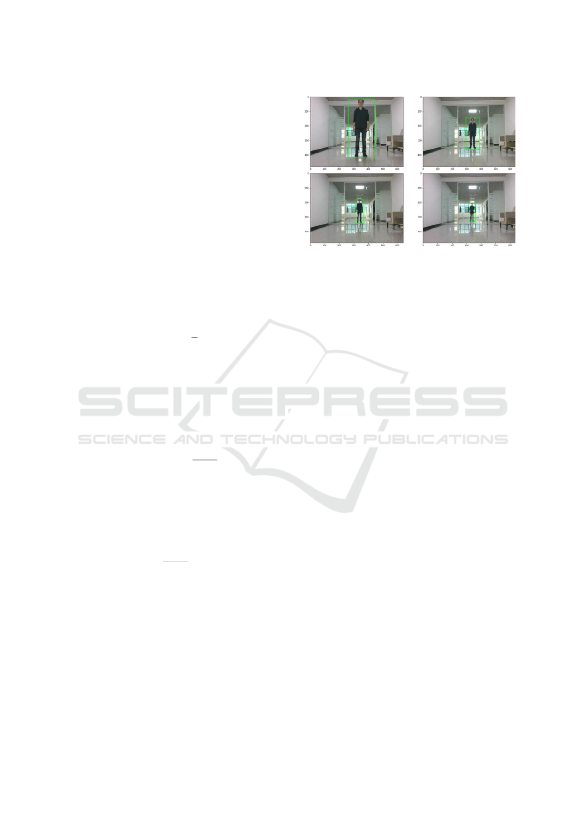
Figure 4: Person at certain ranges.

study, we use the method which was developed by

Zhengyou Zhang and is based on the use of a ﬂat cal-

ibration object in the form of a chessboard (Zhang,

2000). We use the principles of triangle similarity

to ﬁnd the distance to an object at certain ranges, as

shown in Figure 4. The experimental results are given

in the next section.

5.1 Distance Measurement using Depth

Camera

This section describes another and more accurate

method to estimate the distance to an object using a

depth camera (Draelos and at. al., 2015). The depth

camera is working using the following principle:

1. First, it has an Infra-Red(IR) projector that pins

the scene with invisible markers. This allows pro-

jecting Infra-Red lights which pin the object like

a cloud of dots representing the depth for each

pixel. The output of this is called the depth map.

2. The distance triangulation applied between IR

projector and camera.

In simple words, a depth map is an image in

which, for each pixel, instead of color, its distance

from the camera is stored. In our study, we take the

depth map from the Intel depth camera, but it could

also be constructed from a stereo pair of images.

The quality of the depth of an image is highly cor-

related with the resolution of a camera. Our depth

camera supports a few deﬁned depth resolution pre-

sets, which can be selected in advanced camera mode.

We have tried several of them and decided to use

848 × 480. Generally, the lower resolutions can also

be used, but it will decrease the depth precision.

The overall process of ﬁnding the distance to an

object using the depth camera is pretty straight for-

ward. The method that we used consists of several

Detection of Objects and Trajectories in Real-time using Deep Learning by a Controlled Robot

135

steps. Firstly, we capture the object by accessing its

color component RGB frame and depth frame. The

next step is to align both frames because they must be

accessible from the same physical viewport. Figure

5c illustrates the RGB data and depth data combined

into a single RGB-D image and it can be seen that

images is properly aligned. The process of the depth

alignment further allows using the depth data as any

of the other image channels.

After the process of the depth alignment, it is

possible to use any deep learning algorithm on the

RGB frame to ﬁnd speciﬁc objects. In our case, we

use pre-trained state-of-the-art object detection model

YOLOv3 to recognize and localize the object in the

RGB image and use additional depth data to ﬁnd the

distance to an object (Henry et al., 2012).

It can be seen in Figure 5a, the object is found

using object detection model and marked with the

bounding box. Since we have aligned RGB-D image

it is possible to project the bounding box on the depth

frame as shown in Figure 5b. To be more concrete,

we draw the bounding box on the depth frame using

its coordinates from the RGB frame.

Generally, there exist several approaches to cal-

culate the distance to an object. As one of the ap-

proaches, the distance to the object can be measured

by averaging the depth data inside the bounding box.

The number of experiments shows that this is not a re-

liable method, because some depth pixels are too far

away and can signiﬁcantly affect the result of overall

distance measurement. For this reason, we propose

ﬁrst to ﬁnd the coordinates of the center pixel of the

cropped bounding box. In our case, the coordinates

of the center pixel of the bounding box are already

returned by the YOLOv3 model. There also exists

another popular format for the bounding box, instead

of returning x, y, h, w it returns the coordinates of the

corners of the box. The last step is to extract the depth

using the obtained coordinates. The output is the ﬁ-

nal distance to an object. The results of the distance

measurement are provided in the next part.

5.2 Trajectory Estimation

This subsection describes how to estimate the trajec-

tory of an object and the process of getting the co-

ordinates of this object to plot the distance travelled.

The trajectory is the path that the object follows un-

der the given reference frame (Ciaparrone and at. al.,

2020). As we know in classical mechanics the trajec-

tory is represented as a series of the coordinates. The

trajectory vector can be represented as:

= ((x

, y

), (x

, y

), (x

, y

)...(x

, y

)), (4)

(a) RGB image (b) Depth image

Figure 5: Depth estimation process.

where the vector T

contains the coordinates of an ob-

ject.

In our case, to plot the trajectory, we need to ﬁnd

the distance and the angle of an object with respect to

the LIDAR. As was mentioned, the laser rangeﬁnder

(LRF) returns the distance in the form of scans. If the

distance and the angle are known, it is possible to get

the rectangular coordinates of an object. Obviously,

if the coordinates of an object are known it is possible

to plot its trajectory. We used Hokuyo UTM-30LX

scanning laser rangeﬁnder. The LIDAR has a 270

◦

area scanning range with 0.25

◦

angular resolution. In

order to obtain the coordinates of an object, we con-

vert Polar’s LIDAR data into Cartesian coordinates.

Generally, we must solve a simple problem of a right

triangle problem with a known long side and angle.

This allows us to localize an object on the Cartesian

plane. Below are standard formulas for converting a

Polar Coordinates (r,θ ) to Cartesian coordinates (x,y).

radius

= α

degrees

180

(5)

x = r ×cos(α

radius

), y = r × sin(α

radius

) (6)

In the previous sections, the process of detecting an

object and estimating its distance is described. Now,

if the distance to an object and the angle to the object

are known, it is possible to localize the object using

the conversion formula. For example, if the person

stays at 2 meters from LIDAR at an angle of 90

◦

. To

be more accurate, we convert meters to millimetres

and multiplied the result to the re-scaling coefﬁcient

0.05. Then, the coordinates of the person are:

x = (2000 × 0.05) × cos(α

radius

) = 0.079 (7)

y = (2000 × 0.05) × (−sin(α

radius

)) = −99.99 (8)

ROBOVIS 2020 - International Conference on Robotics, Computer Vision and Intelligent Systems

136

As mentioned before, our LIDAR has a scanning

range of 270

◦

, and its angular resolution is 0.25

◦

, so

in total, we have 1080 laser scans, one scan at each

step of angle. In order to simplify the visualization

of the laser beams and to draw a trajectory, we pre-

computed some useful values for plotting trajectory

using the formula below:

radius

= (

−270

value

1080

× 270) ×

180

(9)

where value is the number in the range of 1 and 1080.

Finally, we have obtained an array of radians with

the length of 1080 for the angles between (-135, 135)

which allows us to convert the coordinates by mul-

tiplying the radians obtained at each corresponding

laser scanning range. We visualize the laser beams

using the precalculated values and the canvas library.

The experimental results of the object trajectory are

provided in the following section.

6 EXPERIMENTS AND RESULTS

In this section, we present the datasets used for our ex-

periments. We then describe the experimental results

of the distance measurement. Finally, we present the

results of LIDAR and object detection for the trajec-

tory estimation and the fusion of these two. All the

experiments related to object detection were carried

out on a machine with an Intel Core-i7 8570H pro-

cessor, an NVIDIA GeForce 1080Ti GPU and on an

Ubuntu 16.04 LTS operating system.

6.1 Dataset for Object Detection

There are many publicly available image datasets

used for training models for object detection (Deng

and at. al., 2009). Google Open Images-v4 and Pascal

Visual Object Classes (VOC) 2007 and 2012 are two

of the most popular ones. The Google open images-

v4 dataset contains around 600 classes and 1,743,042

training images, as well as validation 41,620 and

125,436 test images (Kuznetsova and at. al., 2018).

We choose four classes (Person, Box, Chair, Mechan-

ical Fan), which are relevant to our research from

Google’s open image dataset. For testing, we use 10%

of each class and all are high-quality images with dif-

ferent image sizes. The other dataset that we use in

our experiments is the Pascal VOC dataset. The com-

plete dataset contains 20 classes. We merged the Pas-

cal VOC 2007 dataset with 2012. We extracted 12

classes relevant to our study. These classes are air-

plane, bicycle, bus, car, cat, cow, dog, motorcycle,

person, horse, sofa and train.

The training process is done on NVIDIA 1080

Ti GPU. Instead of training model from scratch, we

use pre-trained convolutional weights that have been

trained on the ImageNet dataset. Using these con-

volutional weights helps us to train our model faster.

Additionally, the mean average precision of the model

increases compared to training from scratch.

We trained several YOLO models on our datasets.

The training process for the Pascal VOC dataset took

approximately 5 days for YOLOv3 with an ImageNet

backbone that contains an additional 53 convolutional

layers. The next model to be trained is YOLOv3-tiny.

The training process for the tiny version took about 2

days with the backbone of an ImageNet that contains

15 additional convolutional layers. The average accu-

racy per class is computed every 5000 iterations. In

order to test the algorithm in real-time, we choose the

trained weights with the highest mAP.

6.2 Distance Measurement to the Object

The trained checkpoints of the model allow us to de-

tect and identify the objects in real-time. After the

object is marked with a bounding box, it is possible to

ﬁnd the distance using the methods described earlier.

To evaluate the distance measurements, we conduct

experiments with the class person at 2.75, 5.5, 7.25

and 9 meters from the camera and LIDAR. We com-

pare our results obtained for distance measurement

with similar studies. The results are presented in Ta-

ble 1. The abbreviations used are AD (actual depth),

MD (measured depth) and DERR (depth error rate).

DERR, where Z is the actual depth and Z

indicates

the estimated depth, is calculated as follows.

DERR =

|Z − Z

(10)

The results show that the depth camera has accu-

rate results up to 5 meters. The depth precision start

ﬂuctuates at longer distances. The main advantage

of the depth camera is that it is suitable for the real-

time distance estimation while the monocular real-

time camera ﬂuctuates enormously even at a closer

range. Conventional methods work better at lower

ranges, while LIDAR can give a very precise distance

up to 30 meters with a small deviation in millime-

ters. Table 2 provides accuracy of our approach for

distance measurement and compared to other existing

methods. Algorithm 2 includes the details of distance

measurement using depth camera.

Detection of Objects and Trajectories in Real-time using Deep Learning by a Controlled Robot

137

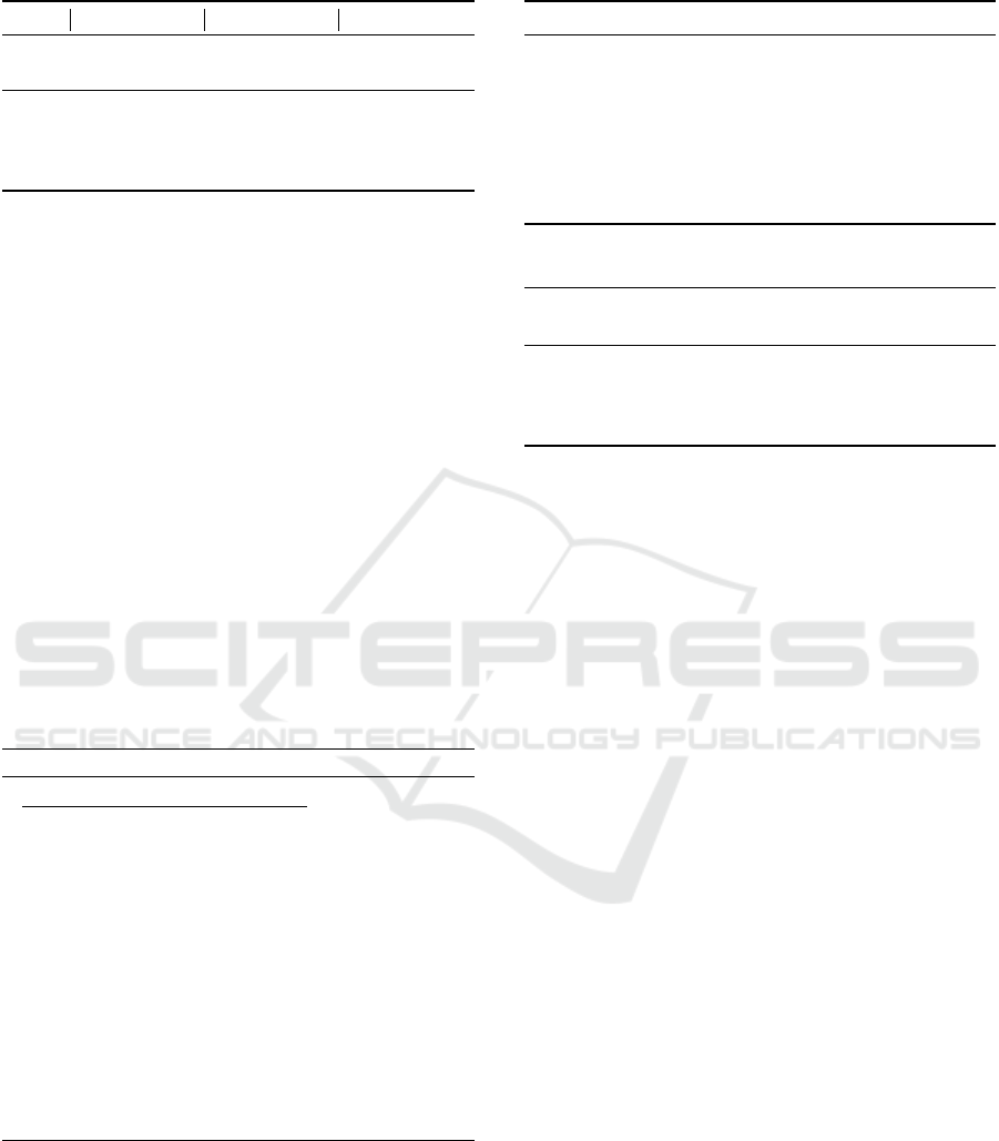
Table 1: Comparison of distance measurement methods.

CMOS Camera Depth Camera 2D LIDAR

(m)

DERR

(%)

(m)

DERR

(%)

(m)

DERR

(%)

2.75 3.02 9.8 2.745 0.18 2.75 0

5.50 4.99 9.2 5.86 6.36 5.50 0

7.25 6.5 10.3 8.1 11.72 7.25 0

9.00 8.01 11 10.2 13.33 9.00 0

6.3 Object Detection and Trajectory

Plot

Now, we give a detailed account for the combination

of the object recognition with LIDAR localization.

The main steps of the algorithm used in our experi-

ments are given below.

1. Detect and recognize an object using YOLOv3.

2. If an object is recognized, then start saving the

coordinates in CSV ﬁle.

3. Plot the trajectory scatter plot of coordinates.

4. Apply polynomial regression in order to smooth

the trajectory path.

The ﬁrst step requires the execution of YOLOv3

in real-time for object detection, since we have al-

ready trained the YOLOv3 model, we can use our

trained weights in order to more precisely detect ob-

jects, which is called transfer learning.

Algorithm 2: Dist. Measurement Using Depth Cam.

function distanceMesurementDepth (V, D, t

);

Input: V : video stream

D : depth stream

: threshold

Output: distance : distance to an object

for each frame f

, f

in V, D do

//detect objects in frame above threshold

detections = detect (f, t

= 0.5)

//draw bounding boxes on detected objects

image = drawBoundingBox(detections, f

)

//reproject bounding boxes on depth frame

depthBoundBox=reprojectBoundBox (detec–s, f

)

//evaluate distance

distance=takeCenterPixel(depthBoundBox)

end

return distance

It is possible to take the minimum range value at

LRF from the ranges at each index of an array of the

scans to verify the closest object at a particular an-

gle. When the object is marked with the bounding

box and begins to move around, its coordinates are

stored continuously in the CSV ﬁle, for further pro-

cessing. Additionally, it is possible to apply a poly-

nomial regression in order to smooth the trajectory.

Table 2: Comparison with the other works.

System Error(%)(Accuracy)

M. Sereewattana et al.(Only for

stationary object below 3m)

3.9 ~12.4

Insu Kim and Kin Choong Yow

(Kim and Yow, 2015)

0.4 ~14.5

CMOS Camera Using Principle of

Similar Triangles

9.2 ~11

Depth Camera 0.18 ~13.33

Laser rangeﬁnder 0

Table 3: RMSE, R

scores for trajectories.

Figure 6 RMSE R

Polynomial

Degree

a 1.62 0.99 10

b 4.9 0.98 5

c 1.95 0.99 4

d 10.92 0.65 3

Polynomial regression ﬁnds the line that best ﬁts our

generated data. Figure 6 shows the various trajecto-

ries for objects and the results of applying polynomial

regression. Table 3 includes corresponding root mean

squared error (RMSE), R

scores and the degree of

each line that best ﬁts to the points.

We have done some experiments to plot the tra-

jectory of a person using the angles obtained from

the LIDAR and the distances obtained from the depth

camera. In addition we compared the trajectories us-

ing distances obtained from the LRF and depth cam-

era in the same angles extracted from the LRF. For

this experiment, a person is moving with a stable 0.5

m/s straight ahead to the LRF and camera, covering

the distance of the about 6.5 meters. Furthermore,

we consider the trajectory obtained from the LRF as

the ground truth. The distances from the depth cam-

era are sufﬁciently accurate and the distribution of the

points is almost the same compared to LRF in a real-

time system. The Y-axis values of the trajectory using

the depth camera are slightly higher than the trajec-

tory using the LRF. It can be concluded that distances

from the depth camera can also be used for detection

of trajectories.

The trajectory is detected by using an ordi-

nary Complementary Metal Oxide Semiconductor

(CMOS) camera. The distribution of coordinates is

very huge because the distances obtained with the

CMOS camera are highly ﬂuctuating. It can be con-

cluded that the single CMOS camera using the prin-

ciple of similar triangles is not suitable for accurate

trajectory plotting in real-time. Then we aggregated

trajectories of the three sensors. The series of coor-

dinates obtained from the depth camera are close to

the ground truth, while the coordinates obtained from

ROBOVIS 2020 - International Conference on Robotics, Computer Vision and Intelligent Systems

138

(a) (b)

Figure 6: Depth estimation process.

Table 4: Comparison of trajectories.

Ground Truth

Sensor

Sensors RMSE Spearman

Correlation

2D LIDAR

Depth

Camera

52.03 0.98

CMOS

Camera

101.5 0.67

the CMOS camera have a high deviation from rest.

Table 4 describes the results of the trajectory compar-

ison using the RMSE and Spearman's rank correlation

coefﬁcient. As a ground truth value, the coordinates

obtained from 2D LIDAR are used.

6.4 Trajectory using Controlled Mobile

Robot

In the previous sections, we traced the trajectory of

a person moving straight relative to the ﬁxed 2D LI-

DAR. We now look at the trajectory plotting with the

same method but with an extension of a trajectory. By

extension, we mean moving our robot to the particular

checkpoint and continuing to calculate the trajectory

of a person with the same technique. The checkpoint

is where the person disappears from the view of the

camera. The pseudo-code of object localisation and

detection of trajectories is given in Algorithm 3.

The experiments have been carried out inside the

building, the same as the previous experiments. In

this speciﬁc experiment, a person is moving with a

stable 0.5 m/s straight ahead from the LRF and the

camera, covering the distance of about 6.5 meters. To-

wards the end of the 6.5 meters, the person is moved

to the right and disappears from the view of the cam-

era. Then our robot moves to this position where the

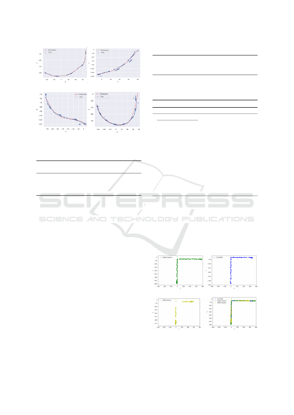
Table 5: Comparison of trajectories.

Ground

Truth

Sensor

Sensors RMSE Spearman

Correlation

2D LIDAR

Depth

Camera

33.37 0.90

CMOS

Camera

78.94 0.61

Algorithm 3: Object Localisation and Trajectory Plot.

function plotTrajectory (V);

Input: V : video stream

Output: coordinates

plot

, regression

plot

: Trajectory plots

for each frame f in V do

//Start saving coordinates of detected object

if Object is in f then

lidar = turnOn()

//get converted coordinates

x, y = lidar.saveCoordinates()

//Stop prog., apply regr–n and plot the traj.

if button “ESC” isPressed then

lidar = turenOff()

coordinates

plot

=plotTrajectory(x, y)

regression

plot

=polynomialRegression(x, y);

end

return coordinates

plot

, regression

plot

person disappears and continue to calculate the trajec-

tory again. The trajectory is shown in Figure 7.

As it is possible to see from this plot, the person

moves straight and turns right, again covering the dis-

tance of about 6.5 meters. Table 5 describes the re-

sults of the trajectory comparison for the case with

the relocation of the mobile robot. It can be concluded

that the trajectory of an object can be estimated using

a mobile robot in a controlled manner.

(a) Trajectory using the Depth camera (b)Trajectory using the LRF

Figure 7: Trajectories of a pedestrian.

Detection of Objects and Trajectories in Real-time using Deep Learning by a Controlled Robot

139

7 CONCLUSION AND FUTURE

WORK

The main objective of this study was to implement

the method for the object trajectory estimation using

the YOLOv3 object detector algorithm an 2D laser

rangeﬁnder. We analysed the YOLOv3 and YOLOv3-

tiny deep learning models on various classes from

datasets including Pascal VOC and Google Open Im-

ages. We used additional pre-trained convolutional

weights to increase the capability of the model to de-

tect the objects. The combination of the object detec-

tion and 2D LIDAR helps the trajectory estimation of

an object. In addition, we tried to plot the trajectory

by using the distances from the depth camera, CMOS

camera and LRF angles. We also estimated the trajec-

tory of an object using a mobile robot in a controlled

fashion. Furthermore, we used polynomial regression

with the purpose of smoothing trajectory path but only

for suitable cases. The experiments show that our ap-

proach is feasible and robust to obtain the object lo-

cation and further draw the trajectory.

As a possible future work, we plan to investigate

different algorithms for the objects trajectory predic-

tion, as well as methods related to object tracking us-

ing mobile robot control.

REFERENCES

Cabasso, J. (2009). Analog vs. ip cameras. Aventura Tech-

nologies, 1(2):1–8.

Ciaparrone, G. and at. al. (2020). Deep learning in video

multi-object tracking: A survey. Neurocomputing,

381:61–88.

Dalal, N. and Triggs, B. (2005). Histograms of oriented

gradients for human detection. In Proceedings of

CVPR’05, pages 886–893. IEEE Computer Society.

Deng, J. and at. al. (2009). Imagenet: A large-scale hi-

erarchical image database. In IEEE Conference on

Computer Vision and Pattern Recognition, pages 248

– 255.

Draelos, M. and at. al. (2015). Intel realsense=real low cost

gaze. pages 2520 – 2524.

Girshick, R., Donahue, J., Darrell, T., and Malik, J. (2013).

Rich feature hierarchies for accurate object detection

and semantic segmentation. pages 98–136.

He, K. and at. al. (2015). Deep residual learning for image

recognition.

Henry, P., Krainin, M., Herbst, E., Ren, X., and Fox, D.

(2012). Rgb-d mapping: Using kinect-style depth

cameras for dense 3d modeling of indoor environ-

ments. The International Journal of Robotics Re-

search, 31(5):647–663.

Hu, J. and at. al. (2017). Squeeze-and-excitation networks.

Keselman, L. and at. al. (2017). Intel realsense stereoscopic

depth cameras.

Khalifa, A. B., Alouani, I., Mahjoub, M. A., and Amara,

N. E. B. (2020). Pedestrian detection using a moving

camera: A novel framework for foreground detection.

Cognitive Systems Research, 60:77–96.

Kim, D. H. and at. al. (2020). Real-time purchase behavior

recognition system based on deep learning-based ob-

ject detection and tracking for an unmanned product

cabinet. Expert Systems with Applications, 143.

Kim, I. and Yow, K. C. (2015). Object location estima-

tion from a single ﬂying camera. In UBICOMM 2015,

page 95.

Krizhevsky, A., Sutskever, I., and Hinton, G. E. (2012). Im-

agenet classiﬁcation with deep convolutional neural

networks. In Proceedings NIPS’12, pages 1097–1105,

USA.

Kuznetsova, A. and at. al. (2018). The open images dataset

v4: Uniﬁed image classiﬁcation, object detection, and

visual relationship detection at scale.

Li, Z. and at. al. (2018). Large-scale retrieval for medical

image analytics: A comprehensive review. Medical

Image Analysis, 43(10).

Liu, W. and at. al. (2016). Ssd: Single shot multibox detec-

tor.

Lu, Z. (2018). Client- server system for web-based visual-

ization and animation of learning content. PhD thesis,

Darmstadt Univ. of Tech., Germany.

Oztarak, H. and at. al (2016). Efﬁcient active rule process-

ing in wireless multimedia sensor networks. I. Journal

of Ad Hoc and Ubiq. Computing, 21:98–136.

Redmon, J. and at. al. (2016). You only look once: Uniﬁed,

real-time object detection. 32(3):779–788.

Redmon, J. and Farhadi, A. (2018). Yolov3: An incremental

improvement.

Ren, S. and at. al. (2015). Faster r-cnn: towards real-time

object detection with region proposal networks. In

Proceedings of NIPS’15, pages 91–99.

Rincon, L. and at. al. (2019). Adaptive cognitive robot using

dynamic perception with fast deep-learning and adap-

tive on-line predictive control. Advances in Mecha-

nism and Machine Science, 73:2429–2438.

Szegedy, C. and at. al. (2016). Inception-v4, inception-

resnet and the impact of residual connections on learn-

ings.

Tan, C. and at. al. (2018). A survey on deep transfer learn-

ing.

Tian, R. and at. al. (2018). Novel automatic human-height

measurement using a digital camera. 2018 IEEE

BMSB, pages 1–4.

Wang, Y. (2014). Tan analysis of the viola-jones face detec-

tion algorithm. An Analysis of the Viola-Jones Face

Detection Algorithm, 4:128–148.

Wei, P. and at. al. (2018). Lidar and camera detection fusion

in a real time industrial multi-sensor collision avoid-

ance system.

Yang, Y. and at. al. (2020). A trajectory planning method for

robot scanning system using mask r-cnn for scanning

objects with unknown model. Neurocomputing.

Zhang, Z. (2000). A ﬂexible new technique for camera cal-

ibration. IEEE, 22(11):1330–1334.

ROBOVIS 2020 - International Conference on Robotics, Computer Vision and Intelligent Systems

140