
Intelligent Algorithms for Non-parametric Robot Calibration
Marija Turkovi
´
c
1,2
, Marko
ˇ
Svaco
1 a
and Bojan Jerbi
´
c
1 b
1
Department of Robotics and Production System Automation, Faculty of Mechanical Engineering and Naval Architecture,
University of Zagreb, Ivana Lu
ˇ
ci
´
ca 5, Zagreb, Croatia
2
Department of Physics, Faculty of Science, University of Zagreb, Bijeni
ˇ
cka cesta 32, Zagreb, Croatia
Keywords:
Non-parametric Robot Calibration, Neural Networks, Genetic Algorithms, Robot Precision.
Abstract:
In this paper, a novel method for non-parametric robot calibration which uses intelligent algorithms is pro-
posed. The non-parametric calibration should prove very useful, because it does not need to identify the
geometric parameters of the robot as is the case in parametric calibration. Instead, only the position measure-
ments need to be provided. This could potentially lead to a cheaper and faster calibration process which could
simplify its application on different and unique robot geometries. The biggest issue of using neural networks
is that they require a lot of data, while for the process of robot calibration a very limited number of measure-
ments is usually collected. In this experiment, the improvement of the hyperparameters of the neural network
was attempted by using the genetic algorithms. Simulations also showed that the parametric optimization
converges faster and that feed-forward back-propagating neural networks could not correctly simulate the be-
haviour of complex robots, or problems which used small datasets. However, for simple robot geometries and
massive datasets, the neural network successfully simulated the behaviour of the robot. Although the number
of measurements needed was well beyond the scope for real world applications, a few possible improvements
were suggested for future research.
1 INTRODUCTION
Robot calibration is a process which can significantly
improve the accuracy of a robot by correcting its po-
sitioning errors. The main objective is to establish an
accurate mapping between the theoretical model of an
idealized robot and an actual measured position. The
inconsistencies in predicted and realized locations of
a robot are arising from many error sources (for exam-
ple, manufacturing tolerances, wear and tear, trans-
mission errors, compliance and set-up errors).
The most common method of calibration is para-
metric calibration, and it focuses on constructing a
model of a robot and determining the actual param-
eters of the robot, thereby improving the positioning
accuracy. This type of calibration was extensively re-
searched over the past decades and many solutions
have already been given (Gang et al., 2014). The para-
metric calibration has in most cases four basic steps.
First, the geometric model of the robot which de-
scribes the relationship between the robot joint space
and the actuator space is made. Afterwards, the ac-
a
https://orcid.org/0000-0002-6761-4336
b
https://orcid.org/0000-0003-1811-5669
tual robot locations are measured by using an exter-
nal measurement device, which is followed by param-
eter identification based on the differences between
the measured and the expected positions. Finally, the
implementation of the modified geometric model is
made, which provides better positioning of the robot
(
ˇ
Svaco et al., 2014).
In recent years, intelligent optimization tech-
niques such as neural networks and genetic algo-
rithms are increasing in popularity in a variety of ap-
plications. Genetic algorithms were inspired by the
process of evolution and there are many approaches
in the calibration techniques which are making use
of genetic programming to minimize the difference in
the actual and ideal robot positions by identifying the
geometric parameters of a robot.
The differential evolution algorithm proved to be
very effective and robust in the case of a serial-parallel
hybrid robot, and the calibration was giving good re-
sults on the simulation of 15 measurements and all of
the 54 geometrical error parameters were successfully
identified. The precision of the final optimization
function approached the scale of 10
−22
(Wang et al.,
2012). Even with a smaller number of measurements,
the different genetic algorithms were able to com-
Turkovi
´
c, M., Švaco, M. and Jerbi
´
c, B.
Intelligent Algorithms for Non-parametric Robot Calibration.
DOI: 10.5220/0010176900510058
In Proceedings of the International Conference on Robotics, Computer Vision and Intelligent Systems (ROBOVIS 2020), pages 51-58
ISBN: 978-989-758-479-4
Copyright
c
2020 by SCITEPRESS – Science and Technology Publications, Lda. All rights reserved
51

pensate for as much as 87% of the positioning error.
The number of measured points was 12, and the per-
formance of the four different algorithms was com-
pared (Barati et al., 2011). Improved quantum par-
ticle swarm optimization (IQPSO) also proved as an
effective algorithm for the identification of the robot
parameters (Wang et al., 2016). The mean squared
error (MSE) of 260 positions measured by the laser
tracker was 2.80 mm, and after IQPSO optimization,
the MSE was only 0.07 mm. Compared with the or-
dinary particle swarm optimization algorithm (Alici
et al., 2006), the convergence speed was improved by
200%. The genetic algorithm can also be used to es-
tablish and identify the whole geometric model of a
robot (Dolinsky et al., 2007). The mapping between
the ideal and the realized robot positions were based
on a dataset of 30 robot measurements. Another 30
positions were used for the validation of the calibra-
tion and the MSE was improved from 1.85 mm prior
to calibration to 0.77 mm after calibration.
Parametric calibration has fast convergence, the
computation cost is low and the insight into the error
sources is provided. Geometrical errors are usually
the main cause of robot inaccuracy and they are re-
sponsible for up to 90% of the total positioning errors
(Judd and Knasinski, 1990). However, non-geometric
error sources (such as joint compliance errors caused
by the robot weight and the payload, link deflection
errors, backlash in gear transmission and thermal ef-
fects) make a smaller but still a significant contribu-
tion to the positional error of the robot (Elatta et al.,
2004). It is difficult to model these effects paramet-
rically because their number is too great to consider
every one of them, but they can be corrected with
non-parametric calibration. This type of calibration is
independent of the robot model, and one of the meth-
ods used for non-parametric calibration is optimiza-
tion with neural networks. It consists of three basic
steps: measurement and the recording of the real and
expected position of the robot, training and testing
the neural network which simulates the behaviour of
the robot and using the neural network output for the
compensation of the error.
Neural networks were mostly used as an addi-
tional step in the calibration process for compensation
of the non-geometric errors after the kinematic pa-
rameters have been determined (Aoyagi et al., 2010).
The first experiments in using neural networks for
robot calibration started three decades ago, and the
artificial neural network managed to reduce the ab-
solute positioning error by 1/3 for a 6-DOF manip-
ulator (Takanashi, 1990). This was succeeded with
a small dataset of 25 measured points. A Recur-
rent Neural Network (RNN) was also used for both
the simulated and the experimental calibration of a 6-
DOF robot (Xiao-Lin Zhong and Lewis, 1995). Only
the internal joint measurements were used while the
manipulator was in contact with the constraint plane,
which generated the identification equations. A Hop-
field type RNN was used for solving these equations
and kinematic parameters were extracted. In total,
120 points have been used and position accuracy has
been improved to the level of robot repeatability. A
back-propagating neural network was used to com-
pensate the joint transmitting error, but only after the
geometric calibration of the robot (Liu et al., 2007).
The input values for the neural network were joint
angles and the information about the rotation direc-
tion, and the output was the angle by which the mo-
tors should rotate. The number of measured points
was 19, and the robot workspace size was 15 x 15 x
15 cm. Experimental verification showed the MSE
decreased from 3.7 mm prior, to 0.5 mm after the cal-
ibration process. More extensive data was provided
with automated measuring system, which collected
more than 10.000 robot positions and configurations
(Zhao et al., 2019). The two-step calibration process
consisted of a parametric calibration which identified
the geometric parameters, and a non-parametric cali-
bration which identified the nonlinear residual errors
by using deep neural networks. The MSE was re-
duced from 1.81 mm to 0.10 mm. The repeatability
accuracy of the robot was 0.05 mm. Other compensa-
tions of non-parametric effects were made with neu-
ral networks after identification of a robots geometric
parameters by using the extended Kalman filter algo-
rithm (Nguyen et al., 2015) and joint angle division
(Wang et al., 2019). Experimental validations of both
methods confirmed the enhanced position accuracy,
which was increased from 3.59 mm to 0.42 mm in the
first, and from 17 cm to 4.5 cm in the second example.
Shallow neural networks were used on a simu-
lated dataset, which demonstrated the superior perfor-
mance of a non-parametric calibration with a neural
network in comparison with bilinear and fuzzy inter-
polations (Bai and Wang, 2019). The absolute posi-
tion accuracy of a drilling robot was also improved
by using the algorithm based on the extreme learning
machine (Yuan et al., 2018). The input of the neural
network was ideal position of a robot and the output
was positional error measured by a laser tracker. The
robot controller was directed to compensate for the
predicted positional errors. By using this method, the
absolute position was improved by 75.89%. It was
also shown that choosing different hyperparameters
of a neural network could increase the accuracy.
The main advantage of the non-parametric cali-
bration lies in the possibility of simple application to
ROBOVIS 2020 - International Conference on Robotics, Computer Vision and Intelligent Systems
52
many different geometries of a robot, which could po-
tentially lower the cost and time needed for the cali-
bration of tailor-made and unique robots. Since the
geometric model does not have to be taken into con-
sideration, calibration is not limited to a pre-defined
model of a robot. The biggest drawback of this ap-
proach is the neural networks tendency to be data-
hungry and the need for a large amount of measure-
ments. Furthermore, there are many network hyper-
parameters which can be adjusted, and this can gen-
erate unwanted errors if the hyperparameters are not
tuned appropriately for the given optimization prob-
lem.
In this paper, we propose a novel method of an
intelligent algorithm which could further improve the
process of calibration by searching for the best hyper-
parameters of a back-propagating feed-forward neural
network.
2 METHODS
Neural networks are universal approximators for non-
linear functions and their behaviour is loosely mod-
eled in resemblance to the interconnected neurons in a
biological brain, which transmit and process the data.
The problems are usually formulated in a way so that
the loss function (the measure of a discrepancy be-
tween the solution predicted by the network and the
solution which is expected and given by the train-
ing set) is minimized on a training dataset, by using
an optimization function which provides the means
for minimization, for a set number of epochs. The
reason for good performance on the various types of
problems is the usage of different activation functions
which introduce nonlinearities in the algorithm. The
challenge which arises from using neural networks
for the robot calibration is the amount of data needed
for successful optimization. Usually, not many mea-
surements for the calibration process are obtained,
because such measurements are time-consuming and
expensive. This can be partially compensated by
choosing a network architecture and hyperparameters
suitable for the specific problem.
While the non-parametric approach with neural
networks is overshadowed by their usage as an addi-
tional step in parametric calibration, there is little re-
search in their direct applications in the process of cal-
ibration. The objective of this experiment was to show
if neural networks can behave in the same way as the
robot that needs to be calibrated, simulating the ex-
act same errors in the robots resulting orientation and
position. However, no insights can be gained about
the error sources as in a parametric calibration; with
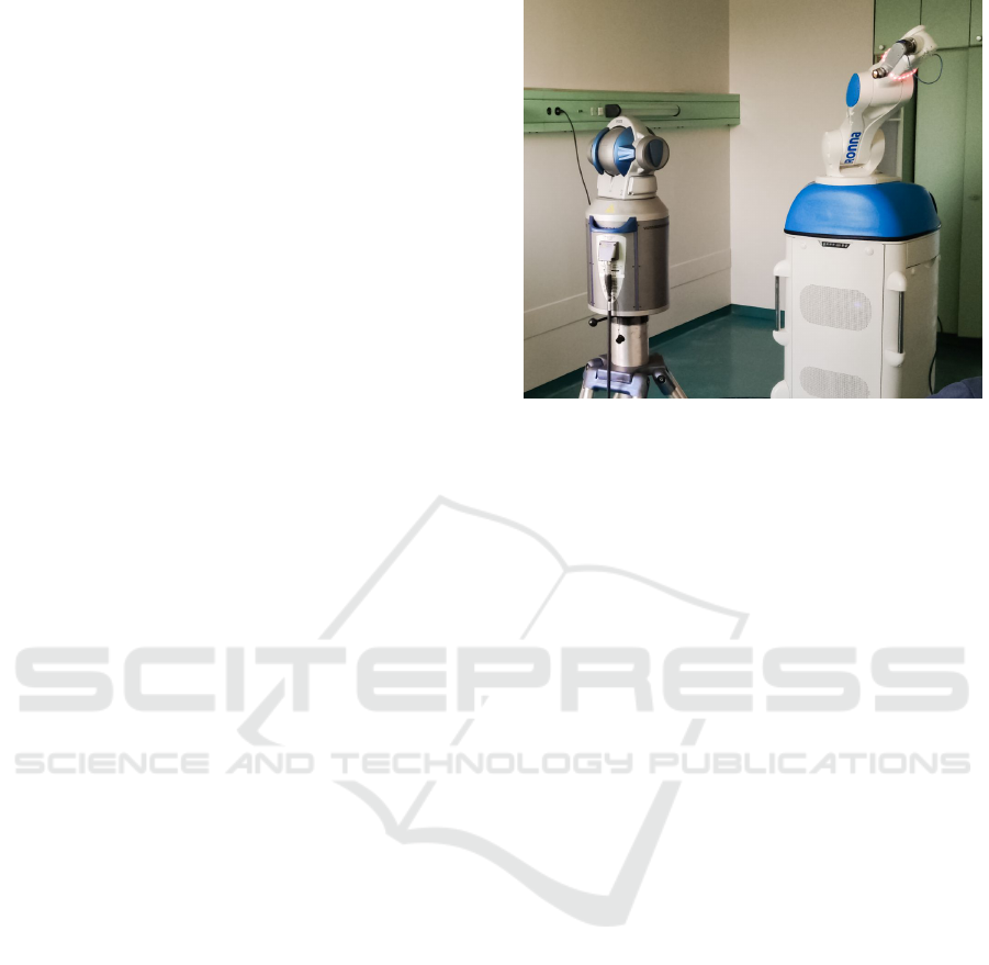
Figure 1: Measurement of the robot positions with a laser
tracker.
its hundreds or thousands parameters neural networks
virtually behave equivalent to a black box because of
the sheer complexity of the code. Unlike the paramet-
ric calibration, this process does not require both the
robot model and the measurements. Instead, only the
measurements should be provided.
The positions of the 6-DOF KUKA KR6 R900
robot were measured with a high-accuracy FARO
ION laser tracker (Figure 1), with the mean per-
centage error of 0.018 mm. The theoretical loca-
tions which the robot was commanded to reach were
recorded as information about the idealized positions
(P
i
), in opposition to measured positions of the robot
(P
m
), and the difference in those two values equals the
robot positioning error. A total of 366 robot positions
were measured. The data was divided into two groups
- the group of idealized positions of the robot (P
i
)
was used as the input for the neural network, and the
group of associated measured positions of the robot
(P
m
) was used as the output for the neural network.
The dataset was then divided into two sets - the train-
ing set with 315 input/output pairs (P
i
, P
m
) and the
test set with 51 input/output pairs (P
i
, P
m
). Every po-
sition P consisted of six values, three of which denote
spatial coordinates (x, y, z) and the other three which
denote the orientation (r, p, y) of the robot.
The neural network used was a feed-forward,
back-propagating network, with two hidden layers
and interconnected neurons in each layer (the number
of neurons was 50). Linear and hyperbolic tangent
functions were used as activation functions, mean ab-
solute error was used for the loss function and the
Adam optimization (Kingma and Ba, 2014) for mini-
mizing the loss function. The learning rate was adap-
tive - the staircase exponential decay was used, and
the input and output pairs were normalized.
Intelligent Algorithms for Non-parametric Robot Calibration
53
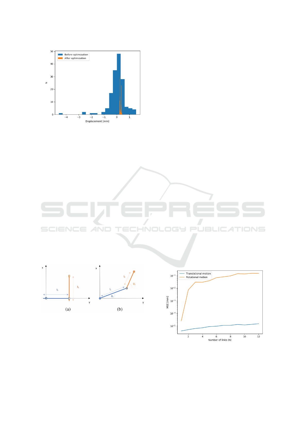
Figure 2: Displacement of the robot manipulator for the
KUKA KR6 R900 before and after optimization.
The distribution of the difference between the
measured (P
m
) and idealized positions (P
i
) for (x, y, z)
components before optimization and the distribution
of the difference between the expected and calculated
positions after the optimization with neural network
was calculated (Figure 2). Although the distribution
of the error after optimization got smaller by an or-
der of magnitude, the error was still quite large. The
reason for such underperformance could perhaps be
found in an inadequate choice of network hyperpa-
rameters.
For the validation of that assumption, the perfor-
mance of the same neural network was then analyzed
on various robot simulations, which were specially
constructed to introduce datasets of robots with var-
ious complexity. The input/output pairs (P
i
, P
m
) were
generated for:
• a planar linear robot with N translational links
• a planar articulated robot with N rotational joints
Figure 3: Schematic representation of the linear (a) and ar-
ticulated (b) planar robots in special case with two links.
The planar linear robot with N links (Figure 3a)
was generated by stacking new links perpendicularly
to the formerly added link. The idealized position (P
i
)
was a set of random x and y positions, while the real-
ized position (P
m
) had an additional constant error (δx
and δy) for every link.
The data for the planar articulated robot with N
links (Figure 3b) was generated by choosing a ran-
dom set of N joint angles (θ
1
, θ
2
, ..., θ
N
) and using the
following equation for the idealized positions P
i
(x, y):
x =
N
∑
i=1
l
i
cos(
i
∑
j=1
θ
i
), y =
N
∑
i=1
l
i
sin(
i
∑
j=1
θ
i
) (1)
The l
i
represents the link length for the ith joint.
For the calculation of the realized robot positions
P
m
(x
error
, y
error
), errors in the link lengths (δl) as well
as errors in the joint angles (δθ) were introduced:
x
error
=
N
∑
i=1
(l
i
+ δl
i
)cos(
i
∑
j=1
(θ
i
+ δθ
i
)) (2)
y
error
=
N
∑
i=1
(l
i
+ δl
i
)sin(
i
∑
j=1
(θ
i
+ δθ
i
)) (3)
With these equations for the linear and articu-
lated planar robots, it was possible to quickly gen-
erate the ”ideal” and ”measured” datasets and to
examine the performance of a former neural net-
work previously used for an optimization of a KUKA
KR6 R900 dataset. The performance of the network
was defined as the mean squared error of the dif-
ference in P
m
(x
error
, y
error
) given by the dataset and
P
0
m
(x
error
, y
error
) predicted by the neural network. The
results were satisfactory in the case with one link for
both robots, but in contrast to the linear robot which
showed good performance (although very slowly de-
creasing as the new links were added), the perfor-
mance of the neural network for the articulated robot
with more than two links significantly decreased by
two orders of magnitude (Figure 4). From this result it
was possible to conclude that the choice of the neural
network hyperparameters used on the specific prob-
lem of the 6-DOF articulated robot was inadequate.
Figure 4: Comparison of the MSE of the linear and the ar-
ticulated robot after optimization.
One of the most challenging tasks will be to de-
termine the best architecture and hyperparameters of
ROBOVIS 2020 - International Conference on Robotics, Computer Vision and Intelligent Systems
54

the neural network for solving the specific calibra-
tion problem when non-linearities are introduced. For
the calibration attempt of the 6-DOF KUKA KR6
R900 robot, another computer-generated model was
created, based on the aforementioned robot.
The robot position is calculated by forward kine-
matics, for which the Denavit-Hartenberg parameters
of the robot (θ, α, d, a) are used. Here, θ stands for the
joint angle of the robot, while α, d and a are inherent
constants which describe the geometry of the robot
and define the robot’s kinematic chain. The model
is also taking into account 24 different kinematic er-
ror parameters (δθ, δα, δd and δa). At the beginning
and the end of the kinematic chain, the robot base ref-
erence frame as well as robot flange reference frame
were added. The position of the robot is calculated by
multiplication of matrix transformations (Jerbi
´
c et al.,
2020):
T = T
base
T
1
T
2
T
3
T
4
T
5
T
6
T
f lange
(4)
Each transformation for the modified Denavit-
Hartenberg notation equals:
T
i
=
cθ
i
−sθ
i
0 a
i
sθ
i
cα
i
cθ
i
cα
i
sα
i
d
i
sα
i
sθ
i
sα
i
cθ
i
sα
i
cα
i
d
i
cα
i
0 0 0 1
, i = 1, ..., 6
(5)
The abbreviations for the sine and cosine func-
tions were used (c = cos and s = sin). The coordinates
and orientations in (P
i
, P
m
) dataset can be calculated
from T .
To find the best hyperparameters of the neural net-
work, the genetic algorithm, which is searching for
the best solution from the population of all potential
solutions, was constructed. At the beginning, a ran-
dom population of the individuals was created. In ev-
ery new generation, the selected individuals are the
best performing ones, and the new possible solutions
were added to the population by recombinations and
mutations of the best-performing individuals. Since
the population is generated completely at random, ge-
netic algorithms have slow convergence speed.
The pseudocode is given as follows:
1: t = 0
2: Population initialization P(t)
3: Evaluation of the population P(t)
4: while (t < T):
5: t = t + 1
6: P’(t) = Selection of the P(t-1)
7: P’’(t) = Mutation of the P’(t)
8: P’’’(t) = Recombination of the P’’(t)
9: Evaluation of the new population P’’’(t)
10: P(t) = P’’’(t)
In this paper we consider the novel method for
robot calibration by using the neural networks care-
fully selected by the genetic algorithm and investigate
its potential in the future usage.
3 RESULTS
The same genetic algorithm was used for both the
parametric and the non-parametric optimization, but
the population for each problem was generated in a
different way. The individual solutions for the para-
metric optimization represented the correction of the
DH parameters used for the calculation of the for-
ward kinematics. Every individual of the population
consisted of 24 numbers in the range of [10
−8
, 10
−2
],
and the data was distributed evenly across the whole
range. The input and output pairs were formed
by computer-generated datasets for the KUKA KR6
R900, and the data was generated for three datasets
with 10, 100 and 1000 pairs of ideal and associated
realized locations of the robot. Best-performing indi-
viduals were selected and added to the new population
by means of crossovers and mutation. A significant
improvement in the accuracy was obtained (Figure 5),
which confirmed the validity of the usage of genetic
algorithms in the parameter identification problems.
Although there were no new insights in using the ge-
netic algorithms in robot calibration, the reference for
the best obtained accuracy was provided, as well as
the time needed for the optimization (Table 1).
Although the number of the individuals in the pop-
ulation was relatively low (30 in each new gener-
ation), all of the three different datasets eventually
reached the satisfactory accuracy. As expected, the
convergence was faster for the largest dataset. Con-
sidering the computation time, a significantly less
time was needed for the dataset with 100 points. The
trade-off for a small increase in precision, as in the op-
timization of the biggest dataset with 1000 robot po-
sitions, means the computation time might be several
times longer. However, with different randomly gen-
erated initial population, the convergence speed could
be a lot faster or slower.
The MSE after optimization was tested on a com-
pletely new dataset specifically created for measuring
the performance of the algorithm, which is the rea-
son the error does not necessarily decrease in time.
Since the generation number varies for every dataset,
for comparison were depicted only the first 1641 gen-
erations (Figure 5), although the datasets with 10 and
100 points also eventually reached the satisfactory ac-
curacy (Table 1).
The non-parametric optimization had a different
Intelligent Algorithms for Non-parametric Robot Calibration
55
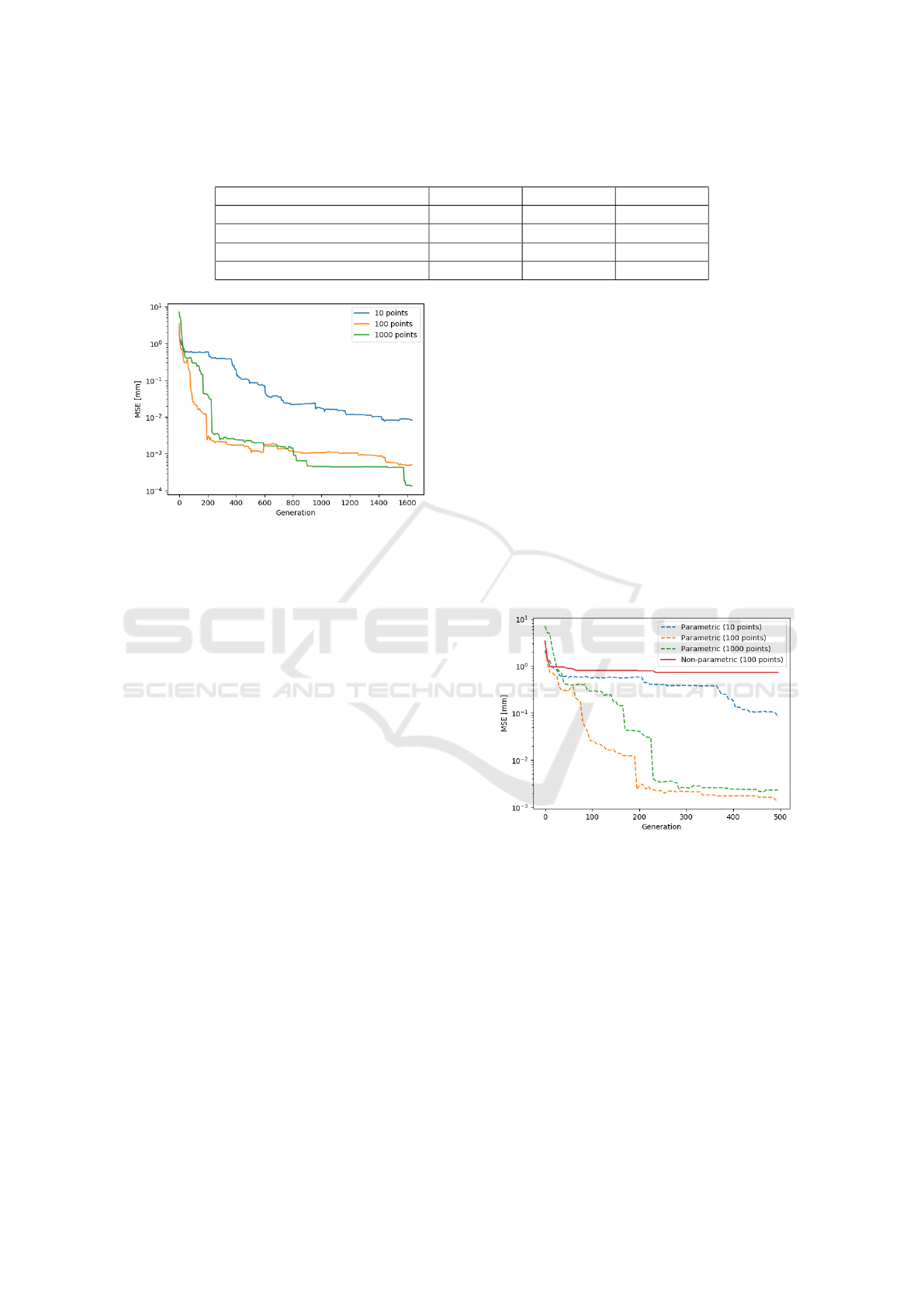
Table 1: The comparison of the mean squared errors after optimization with respect to number of generations and optimization
time for various datasets.
Dataset size 1000 100 10
MSE before optimization [mm] 7.92 8.96 14.26
MSE after optimization [mm] 1.34 × 10
−4
2.04 × 10
−4
5.06 × 10
−4
Number of generations 1641 4451 99996
Optimization time [min] 490 134 366
Figure 5: The behaviour of the mean squared errors for the
parametric optimization by using the genetic algorithm for
three different-sized datasets.
set of initialized population, whose individuals con-
sisted of a variable number of layers, a random num-
ber of neurons for each layer, randomly chosen activa-
tion functions, optimization functions and loss func-
tions. The batch number was also set to random as
well as the normalization range. Sometimes the abil-
ity of the algorithm to generalize well worsens with
time and longer training time does not always guar-
antee better results. For that reason, the number of
epochs of the neural network was also random.
The performance of the different neural net-
work architectures with different hyperparameters
was tested, and the genetic algorithm once again se-
lected the best-performing individuals and added new
population of similar solutions by using crossovers
and mutations. This process seemed very promising
considering the success of both the genetic algorithms
and neural networks in robot calibration. However,
because of the duration of the optimization process,
no new improvement was accomplished (Figure 6).
Time needed for reaching the 500th generation was
166 minutes. This would not be considered long given
the significant improvement in accuracy. But in com-
parison to parametric calibration, the search for the
best neural network architecture was underperform-
ing. The mean squared error for the best-ranked neu-
ral network after 500 epochs was 0.73 mm, and for
the best-ranked parametric calibration for the 10, 100
and 1000 points were 5.06 × 10
−4
mm, 2.04 × 10
−4
mm and 1.34 × 10
−4
mm, respectively.
The reason for this might be found in the be-
haviour of the loss function in the parametric space.
It was generally believed that neural network should
search for global optima and the local optima solu-
tions were not seemed as important. However, the
new research is starting to show that the parametric
space is very densely populated by a large number
of local minima which give results almost as good
as those of the global minimum (Kawaguchi et al.,
2019). No matter what parameters we choose, there
is a great probability the neural network’s solution
found in the local minima will be good enough for
practical applications. In this light, the usage of the
genetic algorithm for choosing the right neural net-
work architecture is not the best way the robot cali-
bration could be done.
Figure 6: The comparison of the MSE for the parametric
and non-parametric optimization.
Since the attempt at the optimization did not
reach the expected values (Figure 2), and no new in-
sights into the architecture of the neural network were
gained, the validity of the usage of neural networks
for optimization in robot calibration was questioned.
The generated input and output pairs (P
i
, P
m
) for the
KUKA KR6 R900 robot were used for verification of
the universal approximation theorem, which claims
that the neural networks should be able to approxi-
mate arbitrary and continuous non-linear functions to
any desired accuracy (Kidger and Lyons, 2019). To
verify this theory, the random neural network archi-
tecture was generated, as well as the data in certain
ROBOVIS 2020 - International Conference on Robotics, Computer Vision and Intelligent Systems
56
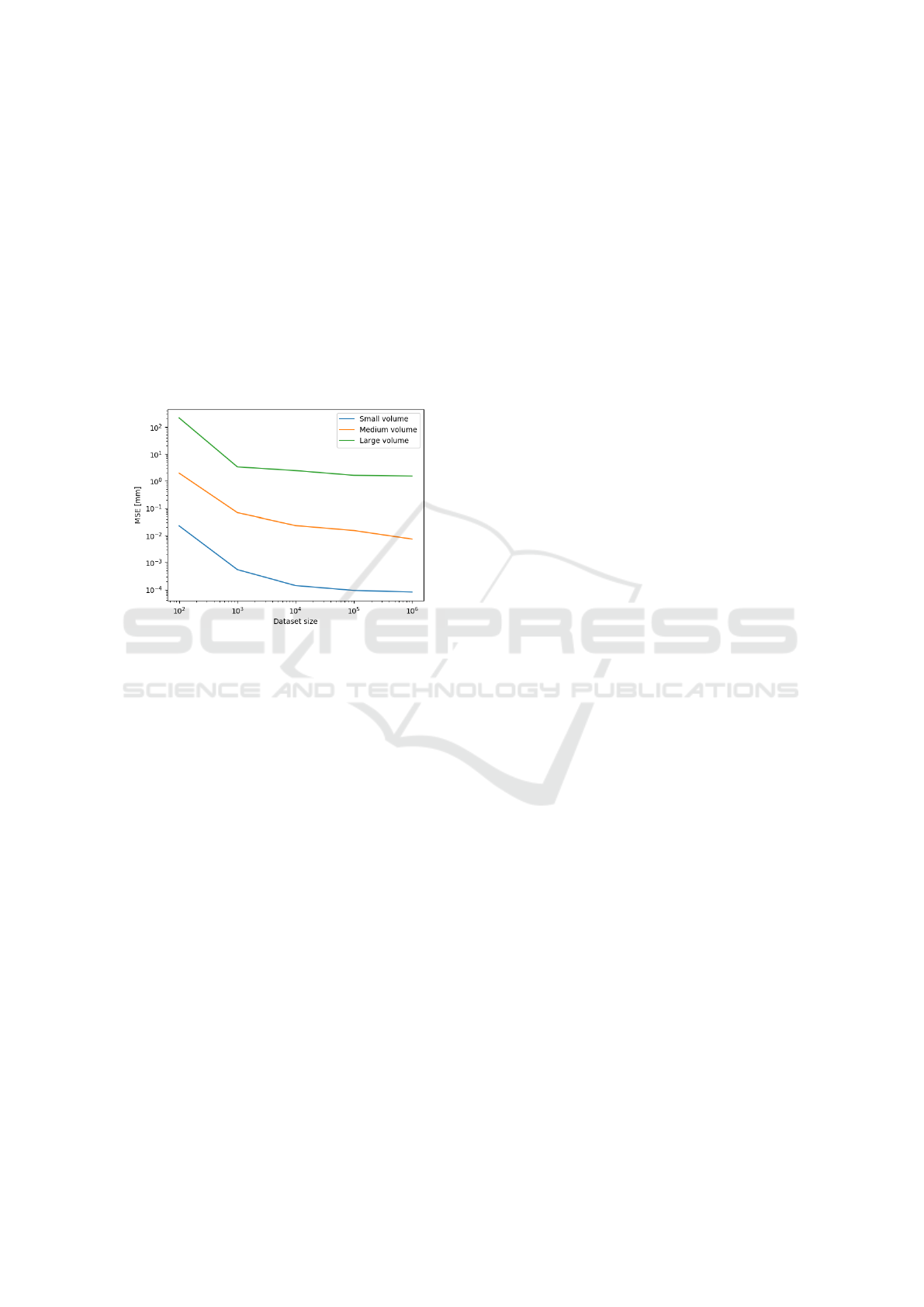
volume range. For the first dataset, the points were
generated in the 2m
3
volume. For the second dataset,
the points were generated in the 2dm
3
volume, and
for the third dataset in the 2cm
3
volume. The various
dataset sizes were used.
The randomly chosen parameters of the neural
network were generated, and the theorem was con-
firmed - the neural network reached the desired accu-
racy for the dataset in the small volume because of the
largest density of the data (Figure 7). With more data,
the optimization process would perform even better.
However, for the purpose of the non-theoretical robot
calibration, the number of measured points should be
below four-digit number.
Figure 7: The behaviour of the MSE with respect to the size
of the input and output datasets, for different volumes.
4 DISCUSSION AND
CONSLUSION
Since the non-parametric robot calibration by using
neural networks was sparsely researched, the possi-
bility of calibration was immediately tested on the
KUKA KR6 R900 robot. The usage of the neural net-
works in the calibration problems showed unsatisfac-
tory results in simulating the behaviour of a 6-DOF ar-
ticulated robot. For that reason, computer-simulated
datasets for two planar robots with different complex-
ities were generated. For the linear robot the cali-
bration proved possible, as opposed to the articulated
robot for which the optimization proved impossible as
soon as additional complexity was introduced.
There are many hyperparameters of the neural net-
work which can be tuned. Otherwise the network
does not produce good approximations for the given
optimization problem. In this paper, a novel method
which uses the genetic algorithms to find an appro-
priate network architecture was proposed, since the
choice of appropriate hyperparameters is of extreme
importance.
Besides the non-parametric, a parametric-
optimization method was tested for reference. The
genetic algorithm was also used, but in this case, the
population consisted of the geometric parameters
which were needed to be identified. The comparison
of the non-parametric and the parametric optimiza-
tion was made on a simulated dataset, and the faster
convergence and better performance of the parametric
optimization was demonstrated.
The validity of the non-parametric calibration at-
tempt was also questioned and tested with massive
datasets. For massive datasets, the feed-forward back-
propagating neural network proved as a good opti-
mizer. However, for the simulation of the complex
robot behaviour, more specific types of network struc-
tures should be researched. Preferably, the number of
the measured positions should be as small as possible
to speed up both the measuring and the calibration
process, but large enough for the model to be able
to generalize well on the whole working space of the
robot.
The solutions considered in this paper are time-
invariant, which does not hold true for the real robot.
Because of the possibility for some manipulators to
reach certain points by alternative joint configura-
tions, the positional errors will be different. It should
prove valuable to consider, in the future research, how
the former movement of the robot affects the error and
if it is possible to make a correction with the neu-
ral networks. By using recurrent networks such as
the LSTM (Long Short-Term Memory), which pro-
cess entire sequences of data, it might be possible to
address this issue. The use of Bayesian Neural Net-
works might also produce better approximations on
smaller datasets because they could extract more in-
formation than other neural networks.
REFERENCES
Alici, G., Jagielski, R., Sekercioglu, A., and Shirinzadeh,
B. (2006). Prediction of geometric errors of robot ma-
nipulators with particle swarm optimisation method.
Robotics and Autonomous Systems, 54:956–966.
Aoyagi, S., Kohama, A., Nakata, Y., Hayano, Y., and
Suzuki, M. (2010). Improvement of robot accuracy
by calibrating kinematic model using a laser tracking
system-compensation of non-geometric errors using
neural networks and selection of optimal measuring
points using genetic algorithm. In 2010 IEEE/RSJ In-
ternational Conference on Intelligent Robots and Sys-
tems, pages 5660–5665.
Bai, Y. and Wang, D. (2019). Using Shallow Neural Net-
work Fitting Technique to Improve Calibration Accu-
racy of Modeless Robots, pages 623–631.
Intelligent Algorithms for Non-parametric Robot Calibration
57

Barati, M., Khoogar, A., and Nasirian, M. (2011). Esti-
mation and calibration of robot link parameters with
intelligent techniques. Iranian Journal of Electrical
and Electronic Engineering, 7:225–234.
Dolinsky, J., Jenkinson, I., and Colquhoun, G. (2007). Ap-
plication of genetic programming to the calibration of
industrial robots. Computers in Industry, 58:255–264.
Elatta, A., Gen, L., Zhi, F., Daoyuan, Y., and Fei, L. (2004).
An overview of robot calibration. Information Tech-
nology Journal, 3:74–78.
Gang, C., Tong, L., Ming, C., Xuan, J. Q., and Xu, S. H.
(2014). Review on kinematics calibration technology
of serial robots. International Journal of Precision
Engineering and Manufacturing, 15:1759–1774.
Jerbi
´
c, B.,
ˇ
Svaco, M., Chudy, D.,
ˇ
Sekoranja, B.,
ˇ
Suligoj,
F., Vidakovi
´
c, J., Dlaka, D., Vitez, N.,
ˇ
Zupan
ˇ
ci
´
c, I.,
Drobilo, L., Turkovi
´
c, M.,
ˇ
Zgalji
´
c, A., Kajtazi, M.,
and Stiperski, I. (2020). RONNA G4 — Robotic neu-
ronavigation: A novel robotic navigation device for
stereotactic neurosurgery. In Handbook of Robotic
and Image-Guided Surgery, pages 599 – 625. Elsevier.
Judd, R. P. and Knasinski, A. B. (1990). A technique to
calibrate industrial robots with experimental verifica-
tion. IEEE Transactions on Robotics and Automation,
6(1):20–30.
Kawaguchi, K., Huang, J., and Kaelbling, L. (2019). Every
local minimum value is the global minimum value of
induced model in nonconvex machine learning. Neu-
ral Computation, 31:1–31.
Kidger, P. and Lyons, T. (2019). Universal approximation
with deep narrow networks.
Kingma, D. and Ba, J. (2014). Adam: A method for
stochastic optimization. International Conference on
Learning Representations.
Liu, J., Zhang, Y., and Li, Z. (2007). Improving the po-
sitioning accuracy of a neurosurgical robot system.
Mechatronics, IEEE/ASME Transactions on, 12:527
– 533.
Nguyen, H.-N., Zhou, J., and Kang, H.-J. (2015). A cali-
bration method for enhancing robot accuracy through
integration of an extended Kalman filter algorithm
and an artificial neural network. Neurocomputing,
151:996–1005.
Takanashi, N. (1990). 6 DOF manipulators absolute
positioning accuracy improvement using a neural-
network. In EEE International Workshop on Intelli-
gent Robots and Systems, Towards a New Frontier of
Applications, pages 635–640 vol.2.
ˇ
Svaco, M.,
ˇ
Sekoranja, B.,
ˇ
Suligoj, F., and Jerbi
´
c, B. (2014).
Calibration of an industrial robot using a stereo vision
system. volume 69, page 459–463.
Wang, F., Wang, Y., Li, J., and Fang, W. (2016). Kinemat-
ics Parameters Identification for IRB 1400 Using Im-
proved Quantum Behaved Particle Swarm Optimiza-
tion, volume 386, pages 881–890.
Wang, Y., Wu, H., and Handroos, H. (2012). Error
modelling and differential-evolution-based parameter
identification method for redundant hybrid robot. In-
ternational Journal of Modelling and Simulation, 32.
Wang, Z., Chen, Z., Wang, Y., Mao, C., and Hang, Q.
(2019). A robot calibration method based on joint an-
gle division and an artificial neural network. Mathe-
matical Problems in Engineering, 2019:1–12.
Xiao-Lin Zhong and Lewis, J. M. (1995). A new method
for autonomous robot calibration. In Proceedings of
1995 IEEE International Conference on Robotics and
Automation, volume 2, pages 1790–1795 vol.2.
Yuan, P., Chen, D., Wang, T., Cao, S., Cai, Y., and Xue,
L. (2018). A compensation method based on extreme
learning machine to enhance absolute position accu-
racy for aviation drilling robot. Advances in Mechan-
ical Engineering, 10:168781401876341.
Zhao, G., Zhang, P., Ma, G., and Xiao, W. (2019).
System identification of the nonlinear residual er-
rors of an industrial robot using massive measure-
ments. Robotics and Computer-Integrated Manufac-
turing, 59:104–114.
ROBOVIS 2020 - International Conference on Robotics, Computer Vision and Intelligent Systems
58
