Computation of Neural Networks Lyapunov Functions for Discrete and
Continuous Time Systems with Domain of Attraction Maximization
Benjamin Bocquillon
1
, Philippe Feyel
1
, Guillaume Sandou
2
and Pedro Rodriguez-Ayerbe
2
1
Safran Electronics & Defense, 100 avenue de Paris, Massy, France
2
Universit
´
e Paris-Saclay, CentraleSup
´
elec, CNRS, L2S, 3 rue Joliot Curie, 91192 Gif-Sur-Yvette, France
Keywords:
Lyapunov Function, Domain of Attraction, Optimization, Neural Network, Nonlinear System.
Abstract:
This contribution deals with a new approach for computing Lyapunov functions represented by neural net-
works for nonlinear discrete-time systems to prove asymptotic stability. Based on the Lyapunov theory and
the notion of domain of attraction, the proposed approach deals with an optimization method for determin-
ing a Lyapunov function modeled by a neural network while maximizing the domain of attraction. Several
simulation examples are presented to illustrate the potential of the proposed method.
1 INTRODUCTION
Lyapunov theory, introduced in the late nineteenth
century (Lyapunov, 1892), is a classical way to in-
vestigate for the stability of an equilibrium point for
a dynamical system. The method relies on the search
for a function that exhibits three important properties
that are sufficient for establishing the Domain Of At-
traction (DOA) of a stable equilibrium point : (1) it
must be a local positive definite function; (2) it must
have continuous partial derivatives, and (3) its time
derivative along any state trajectory must be negative
semi-definite. Although efficient to prove stability
once the so-called Lyapunov function is known, there
is no general method for constructing such a function.
The Lyapunov function construction is still an
open problem, but several methods, often based on
optimization, have emerged in the literature. One can
cite (Panikhom and Sujitjorn, 2012), where the best
quadratic Lyapunov function is looked for. However,
these methods are too conservative in case of indus-
trial complex systems. The work of (Arg
´
aez et al.,
2018) proposes a new iterative algorithm that aims
to avoid obtaining trivial solutions when construct-
ing completive Lyapunov functions. This algorithm
is based on mesh-free numerical approximation and
analyses the failure of convergence in certain areas
to determine the chain-recurrent set. Once again, the
method appears too difficult for being used in an in-
dustrial context where flexibility is needed. Finally,
the survey (Giesl and Hafstein, 2015) has brought dif-
ferent methods and gave a wide overview of the meth-
ods that can be used for the Lyapunov function com-
putation. It proposes conservative methods when the
system is complex and highly non-linear.
However, to the authors’ mind, Artificial Intelli-
gence, Machine Learning and Neural Network bring
a great opportunity to design powerful tools to jus-
tify and quickly certificate complex industrial systems
such as in the aerospace field for instance. One of the
first papers using Artificial Intelligence to compute
Lyapunov function is (Prokhorov, 1994), where a so
called Lyapunov Machine, which is a special-design
artificial neural network, is described for Lyapunov
function approximation. The author indicates that
the proposed algorithm, the Lyapunov Machine, has
substantial computational complexity among other is-
sues to be resolved and defers their resolution to fu-
ture work. The work of (Banks, 2002) suggests a
Genetic Programming for computing Lyapunov func-
tions. However, the computed Lyapunov functions
may have locally a conservative behavior. In this
study, the use of Neural Networks allows to overcome
these limits. Neural Networks are known to be pow-
erful regressors that can approximate any nonlinear
function. As a result, they appear as a good candi-
date for the construction of a Lyapunov function. In
the literature, one can find other works using neu-
ral network to construct or approximate a Lyapunov
function (Serpen, 2005) and the paper (Petridis and
Petridis, 2006) where the authors propose an interest-
ing and promising approach for the construction of
Lyapunov functions represented by neural networks.
In (Bocquillon et al., 2020), the authors propose to
use a new constrained optimization scheme such that
the weights of this neural network are calculated in a
way that is mathematically proven to result in a Lya-
punov function while maximizing the DOA.
Bocquillon, B., Feyel, P., Sandou, G. and Rodriguez-Ayerbe, P.
Computation of Neural Networks Lyapunov Functions for Discrete and Continuous Time Systems with Domain of Attraction Maximization.
DOI: 10.5220/0010176504710478
In Proceedings of the 12th International Joint Conference on Computational Intelligence (IJCCI 2020), pages 471-478
ISBN: 978-989-758-475-6
Copyright
c
 2020 by SCITEPRESS – Science and Technology Publications, Lda. All rights reserved
471

Although most of works relative to Lyapunov
computation deal with continuous time systems, only
few ones related to the discrete time case. Numeri-
cal methods to compute Lyapunov functions for non-
linear discrete time systems have been presented, for
example in (Giesl, 2007), where collocation is used
to solve numerically a discrete analogue to Zubov’s
partial differential equation using radial basis func-
tions. For nonlinear systems with a certain structure
there are many more approaches in the literature. To
name one, in (Milani, 2002) the parameterization of
piecewise-affine Lyapunov functions for linear dis-
crete systems with saturating controls is discussed.
However, although effective, these approaches either
look difficult to implement for real complex systems
or are too conservative.
In this paper, we extend the proposition in (Boc-
quillon et al., 2020) dedicated to continuous systems
to the case of discrete-time ones. We enhance the us-
ability of the algorithm by extending this approach for
discrete time systems. Our contribution is to unify
the continuous and discrete time cases towards an ef-
ficient formulation of the optimization problem. Note
that the goal of this study is not to stabilize a given
plant, but to analyze its stability, computing an ap-
proximation of the potential domain of attraction. Our
paper does not deal of the stabilization of the system
itself.
The paper is composed of 4 sections: the first part
is related to the design of neural network Lyapunov
function for the continuous part. The second part,
which is the main contribution of this paper, proposes
an extension to the discrete time case. The third part
is where we present the proposed algorithm to com-
pute a candidate Lyapunov function through optimal
neural network weights calculation while maximizing
the DOA. And the last one describes examples show-
ing efficiency of the paper.
2 CONTINUOUS TIME CASE
2.1 Theoretical Background
Notations and definitions used in the paper are called
in this section. Let R denote the set of real numbers,
R
+
denote the set of positive real numbers, k.k denote
a norm on R
n
, and X ⊂ R
n
, be a set containing X = 0.
Consider the autonomous system given by (1).
˙
X = f (X ) (1)
where f : X → R
n
is a locally Lipschitz map from a
domain X ⊂ R
n
into R
n
and there is at least one equi-
librium point X
e
, that is f(X
e
) = 0.
Theorem 2.1 (Lyapunov Theory) (Khalil and Griz-
zle, 2002). Let X
e
= 0 be an equilibrium point for
(1). Let V : D → R be a continuously differentiable
function,
V (0) = 0 and V (X) > 0 in D − {0} (2)
˙
V (X) ≤ 0 in D (3)
then, X
e
= 0 is stable. Moreover, if
˙
V (X) < 0 in D − {0} (4)
then X
e
= 0 is asymptotically stable.
Where D ⊂ X ⊂ R
n
is called Domain Of Attraction
(DOA) and the system will converge to 0 from every
initial point X
0
belonging to D.
2.2 Neural Network Formalism
The work in this section is based on the approach de-
veloped in the paper (Bocquillon et al., 2020) and is
reported here for sake of clarity.
Let us consider the autonomous system in (1), in
which we assume without any loss of generality, that
the equilibrium point considered for the stability anal-
ysis is the point 0 (X=0). Therefore,
f (0) = 0 (5)
Suppose V(X) is a scalar, continuous and differen-
tiable function and its derivative with respect to time
is given in (6).
G(X) =
dV
dt
=
n
∑
j=1
∂V
∂x
j
f
j
(X) (6)
with X = [x
1
,...,x
n
]
T
.
The Lyapunov function is modeled by a neural
network with a single hidden layer whose weights
are calculated in such a way that is proven mathemat-
ically that the resulting neural network implements
indeed a Lyapunov function, showing the asymptotic
stability in the neighborhood of 0. We assume that
the Lyapunov function V(X) is represented by a
neural network where the x
i
are the inputs, w
ji
are
the weights of the hidden layer, a
i
the weights of the
output layer, h
i
are the biases of the hidden layer, θ
is the bias of the output layer; i=1,...,n and j=1,...,K
where K is the number of neurons of the hidden layer
and σ is the activation function of the neural network.
Therefore, V(X) can be expressed as:
NCTA 2020 - 12th International Conference on Neural Computation Theory and Applications
472

V (X) =
K
∑
i=1
a
i
σ(ν
i
) + θ (7)
ν
i
=
n
∑
j=1
w
ji
x
j
+ h
i
(8)
From (2) and (4), sufficient conditions for the
point 0 of system (1) to be asymptotic stable in the
sense of Lyapunov are:
(a1) V(0) = 0.
(a2) V(X) > 0 for all nonzero X in a neighbour-
hood of 0.
(a3) G(0) = 0.
(a4) G(X ) < 0 for all nonzero X in a neighbour-
hood of 0.
From (a1) and (a2), sufficient conditions for V(X)
to have a local minimum at 0 are (Petridis and
Petridis, 2006):
(v1) V(0) = 0.
(v2)
∂V
∂x
j




X=0
= 0 for all j=1,2,...,n.
(v3) H
V
(the matrix of 2
nd
derivatives of V at X=0)
is positive definite.
In the same way from (a3) and (a4), sufficient con-
ditions for G(X) to have a local maximum at 0 are
(Petridis and Petridis, 2006):
(d1) G(0) = 0.
(d2)
∂G
∂x
j




X=0
= 0 for all j=1,2,...,n.
(d3) H
G
(the matrix of 2
nd
derivatives of G at X=0) is
negative definite.
Then, the second derivative of V(X) and G(X) are
computed as functions of the neural network :
V
qr
=
∂
2
V
∂x
q
∂x
r




X=0
=
K
∑
i=1
a
i
d
2
σ(ν
i
)
dν
2
i




X=0
∂v
i
∂x
r




X=0
w
qi
=
K
∑
i=1
a
i
d
2
σ(ν
i
)
dν
2
i




X=0
w
ri
w
qi
(9)
G
l p
=
∂
2
G
∂x
l
∂x
p




X=0
=
n
∑
j=1
K
∑
i=1
a
i
d
2
σ(ν
i
)
dν
2
i




X=0
w
ji
w
li
!
J
jp
+
+
n
∑
j=1
K
∑
i=1
a
i
d
2
σ(ν
i
)
dν
2
i




X=0
w
ji
w
pi
!
J
jl
(10)
where J
qr
=
∂ f
q
∂x
r




X=0
q=1,...,n; r=1,...,n; l=1,...,n;
p=1,...,n.
Therefore,
H
V
= [V
qr
(X = 0)] V
qr
is given by (9) (11)
H
G
= [G
l p
(X = 0)] G
l p
is given by (10) (12)
Assuming that the Lyapunov function is repre-
sented by a neural network, conditions (v1) - (v3) and
(d1) - (d3) reduce to (we choose here σ(ν) = tanh(ν)):
(t1)
K
∑
i=1
a
i
σ(h
i
)+θ = 0. (13)
(t2)
K
∑
i=1
a
i
(1 − tanh
2
(h
i
))w
qi
= 0 for q=1,...,n.
(14)
(t3) H
V
as given by (11) is positive definite.
(t4) H
G
as given by (12) is negative definite.
We only deal with differentiable activation func-
tions.
3 DISCRETE TIME CASE
3.1 Additional Theoretical Background
Consider the autonomous discrete time system given
by (15).
X(k + 1) = f (X(k)) (15)
where f : X → R
n
is a locally Lipschitz map from a
domain X ⊂ R
n
into R
n
and there is at least one equi-
librium point X
e
, that is f(X
e
) = X
e
.
Computation of Neural Networks Lyapunov Functions for Discrete and Continuous Time Systems with Domain of Attraction Maximization
473

Theorem 2.2 (Lyapunov Theory Discrete Time)
(Khalil and Grizzle, 2002).
Consider the autonomous system given by (15).
Let X
e
= 0 be an equilibrium point for (15). Let
V : D → R be a continuous function,
V (0) = 0 and V (X(k)) > 0 in D − {0} (16)
V (X(k + 1)) −V (X(k)) ≤ 0 in D (17)
then, X
e
= 0 is stable. Moreover, if
V (X(k + 1)) −V (X(k)) < 0 in D (18)
then X
e
= 0 is asymptotically stable.
3.2 Adaptation of the Neural Network
Formalism
Let us consider the autonomous system in (15), in
which we assume that the equilibrium point of interest
for the stability analysis is the point 0. Therefore,
f (0) = 0 (19)
Suppose V (X(k)) the Lyapunov function for the
discrete time case and,
G(X(k)) = V (X (k + 1)) −V (X(k))
(20)
with X(k) = [x
1
(k), ...,x
n
(k)]
T
.
In the discrete time case, sufficient conditions (a1)
- (a4) for the point 0 of system to be asymptotically
stable in the sense of Lyapunov are still the same than
in the continuous part explained above. Conditions
(v1) - (v3) and (d1) - (d3) which prove that V (X(k))
to have a local minimum at 0 and G(X(k)) to have
a local maximum at 0 are also equivalent. However,
the derivative of the function V (X) is not defined in
the same way for the continuous and the discrete time
case. Therefore, in this extension we will present how
to define the new H
G
matrix.
First and second derivatives of G(X(k)) can be calcu-
lated from (20) :
G
l
=
∂G
∂x
l
=
n
∑
h=1
∂V
∂x
h
∂ f
h
∂x
l
−
∂V
∂x
l
(21)
G
l p
=
∂
2
G
∂x
l
∂x
p
=
n
∑
h=1
∂
2
V
∂x
h
∂x
p
∂ f
h
∂x
l
+
n
∑
h=1
∂V
∂x
h
∂
2
f
h
∂x
l
∂x
p
−
∂
2
V
∂x
l
∂x
p
with l = 1,...,n and p = 1,...,n
(22)
In view of condition (v2), (21) and (22) result in,
G
l
(0) = 0 for all l = 1, 2, ..., n (23)
and
G
l p
(0) =
n
∑
h=1
∂
2
V
∂x
h
∂x
p





X(k)=0
∂ f
h
∂x
l




X(k)=0
−
∂
2
V
∂x
l
∂x
p




X(k)=0
(24)
On the basis of (24) we can write,
H
G
= [G
l p
(X(k) = 0)] = H
V
J − H
V
(25)
since H
V
is symmetric. H
G
is a matrix whose ele-
ments are G
l p
(0) and J is the Jacobian of f (X(k)) at
X(k) = 0.
Let us assume that the Lyapunov function,
V (X(k)), is represented by the neural network defined
in (7) and (8). Therefore, the second derivative of
G(X(k)) is computed as functions of the neural net-
work weights,
G
l p
(0) =
n
∑
j=1
(
K
∑
i=1
a
i
∂
2
σ(ν
i
)
∂
2
ν
i
w
ji
w
li
)J
jp
−
n
∑
j=1
(
K
∑
i=1
a
i
∂
2
σ(ν
i
)
∂
2
ν
i
w
ji
w
pi
)
(26)
where J
qr
=
∂ f
q
∂x
r




X(k)=0
q=1,...,n; r=1,...,n; l=1,...,n;
p=1,...,n.
Therefore,
H
V
= [V
qr
(X(k) = 0)] V
qr
is given by (9) (27)
H
G
= [G
l p
(X(k) = 0)] G
l p
is given by (26) (28)
Point X(k) = 0 is asymptotically stable if condi-
tions (t1) - (t4) hold with the new definition of the
matrix H
G
.
4 THE PROPOSED ALGORITHM
4.1 Optimization Scheme
The work in this section is based on the approach de-
veloped in the paper (Bocquillon et al., 2020) and is
reported here for sake of clarity.
First, for an appropriate Lyapunov function to be
NCTA 2020 - 12th International Conference on Neural Computation Theory and Applications
474

determined, values of the weights of the neural net-
work should be calculated such that the conditions
(t1)-(t4) are satisfied. To this end, a cost function,
Q , should be selected so that positivity and negativity
respectively of H
V
and H
G
are constrained. The sym-
metric matrix H
G
is negative definite if all its eigen-
values are negative.
Denote λ
v
i
, i=1,...,n
v
the set of the n
v
eigenvalues
of H
V
and λ
g
i
, i=1,...,n
g
the set of the n
g
eigenvalues
of H
G
.
4.2 DOA Maximization Problem
The work in this section is based on the approach de-
veloped in the paper (Bocquillon et al., 2020) and is
reported here for sake of clarity.
Conditions (a2) and (a4) prove the asymptotic sta-
bility only ”in a neighbourhood of 0”. Consider that a
Lyapunov function V(X) is given, by definition of D in
(2) and (3), the system will converge to 0 from every
initial point X
0
belonging to D. Thus, to maximize
the DOA we search for an approximation
ˆ
D as large
as possible, where the system is stable. Therefore,
ˆ
D
= D would be the best possible case.
Consider Z a set of points obtained from a hy-
percube whose faces are gridded in order to cover a
sufficiently large enough domain ⊂ X. Note that, Z
has to be chosen large enough such as it contains D.
We denote P = max (ratio
v
, ratio
dv
) where ratio
v
are
the number of points X ⊂ Z where evaluated V(X)<
0 and ratio
dv
are the number of points X ⊂ Z where
evaluated
˙
V (X)> 0. In order to maximize
ˆ
D, we have
to minimize P.
Note that, there are other more intelligent methods
to determine the gridding but so far, we used the one
presented previously. For example, in the future, a
possible approach is to use the gradient of the current
Lyapunov function candidate during the optimization.
An idea could be to analyze the first run of the opti-
mization algorithm and the larger the gradient is, the
thinner the gridding has to be in the next runs.
4.3 Constrained Implementation
We now formalize the problem as a constrained one
to avoid the use of barrier function which would
lead to a suboptimal problem (Petridis and Petridis,
2006), whose solution needs to be a posteriori ver-
ified. The scheme proposed here is flexible so that
more complex problems such as exponential stability,
robust stability or Input-to-state stability (ISS), will
efficiently be tackled in future works.
The problem can be expressed in the general form
of an optimization problem in which the cost function
Q needs to be minimized.
To this purpose, we set down:
H
V
0
= H
V
× -1
Denote λ
v0
as the eigenvalues of H
V
0
.
−
λ
v
0
= max(real(λ
v0
))
−
λ
g
= max(real(λ
g
))
−
λ = max (
−
λ
v
0
,
−
λ
g
)
According to (7) and (8), we denote α as the deci-
sion variables where:
α = [w
ji
,a
i
,h
i
,θ] (29)
Then, the cost function to be minimized has the
following form:
min
α
Q
If
−
λ > 0
Q =
−
λ
Else
Q = -
1
P + 1
which is a similar formulation of the cost function
that can be find in (Feyel, 2017) and has proven its
efficiency. According to the definition of the problem
Q , a neural network candidate is a Lyapunov function
if Q < 0. Assuming D ⊂ Z, best case, Q = - 1, refers
to
ˆ
D = D. The P+1 avoids singularities when P = 0.
The benefit of this formulation is its great flexibility:
easy adaptation for a multitude of complex problems,
extension to other type of stability and no additional
parameter to tune for the penalty function. Besides,
we have the guarantee that in the domain
ˆ
D the eigen-
values of H
V
and H
G
have respectively real positive
and negative values. Finally, no parameter is needed.
5 SIMULATION RESULTS
In this section, we apply our approach to one continu-
ous time system and to two different discrete time sys-
tems to validate the extension. For clarity purposes,
we have chosen some two dimensional examples so
that the results can be easily plotted.
The entire test was performed on a machine
equipped with an Intel Core i5 - 8400H (2.5 GHz)
processor and 16 GB RAM.
Computation of Neural Networks Lyapunov Functions for Discrete and Continuous Time Systems with Domain of Attraction Maximization
475

5.1 Parameter Settings
The parameters settings used in the tests are as fol-
lows:
• We consider 1 hidden layer and the number of
neurons of this hidden layer is arbitrarily set to
K = 12.
• In both continuous and discrete time cases, we set
x as a rectangle of 21 × 21 centered at 0. There-
fore, V (X) and
˙
V (X) are evaluated in 441 points
in the range of each system.
• The number of searched variables α (29) is: K ×
(2n) + 1 = 49, and each of them has its search
space interval arbitrarily defined by [-4; 4].
• The optimization method to calculate the weights
of the neural network to compute a Lyapunov
function is the Genetic Algorithm from the Global
Optimization Toolbox in Matlab, used, for in-
stance, in (Krishna et al., 2019). Other parame-
ters that are not mentioned are the default value in
GA, like the mutation rate for instance.
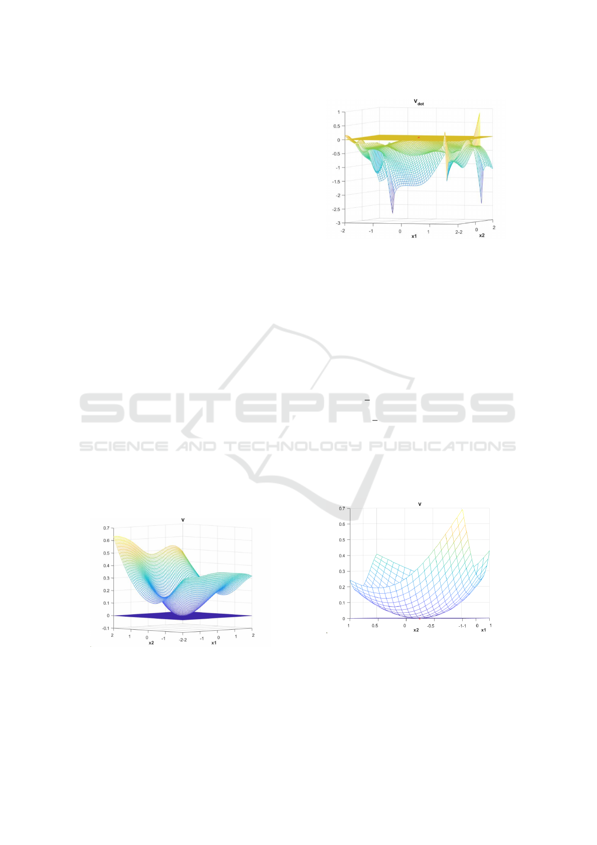
5.2 Continuous Time System
Example 1
Let us consider the following system:
(
˙x
1
= −tan x
1
+ x
2
2
˙x
2
= −x
2
+ x
1
The ranges for x
1
and x
2
are x
1
∈ [−1,1] and x
2
∈
[−1,1]. The stability of the origin is considered and
the Figures 1 and 2 show the result.
Figure 1: The constructed Lyapunov function for this sys-
tem.
The proposed method is compared to the method
from (Banks, 2002), based on genetic programming
techniques. From Figures 1 and 2, we can easily
check that our method provides a larger
ˆ
D than the
Figure 2: The time derivative of the constructed Lyapunov
function.
one found in the paper, which shows the efficiency of
our approach. Therefore, the origin of the system is
asymptotically stable.
5.3 Discrete Time Systems
Example 2
Let us consider the following system:





x
+
=
1
2
x + x
2
− y
2
y
+
= −
1
2
y + x
2
The ranges for x and y are x ∈ [−1,1] and y ∈
[−1,1]. The stability of the origin is considered and
the Figures 3 and 4 show the result. The Figure 4
shows the function V (X(k +1))−V (X(k)) of the sys-
tem.
Figure 3: The constructed Lyapunov function for this sys-
tem.
We can easily check that the underlying function
expressed by the network input-output relation is a
Lyapunov function for this system. Therefore, the ori-
gin of the system is asymptotically stable.
NCTA 2020 - 12th International Conference on Neural Computation Theory and Applications
476

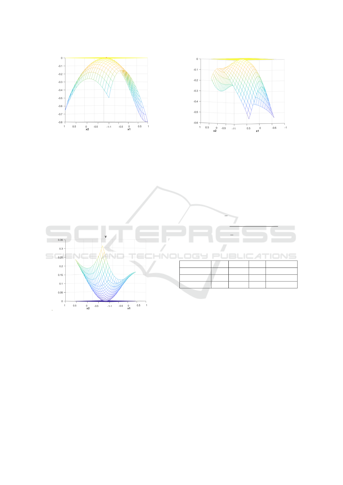
Figure 4: The difference function of the constructed Lya-
punov function.
Example 3
Let us consider the following system:
(
x
+
= −0.125y − 0.125(1 − x
2
− y
2
)x
y
+
= 0.125x − 0.125(1 − x
2
− y
2
)y
The ranges for x and y are x ∈ [−0.75,0.75] and
y ∈ [−0.75,0.75]. The stability of x
e
= [0; 0] is con-
sidered and the Figures 5 and 6 show the result. The
Figure 6 shows the function V (X(k + 1)) −V (X(k))
of the system.
Figure 5: The constructed Lyapunov function for this sys-
tem.
We can easily check that the underlying function
expressed by the network input-output relation is a
Lyapunov function for this system. Therefore, the
equilibrium point x
e
= [0; 0] of the system is asymp-
totically stable.
5.4 Performance Measurement
Since the tested optimization algorithm is stochastic,
a statistical analysis of the results is required. Thus,
the performance measurement rule is as follows.
The cost function Q is defined in the section 4.3.
Figure 6: The difference function of the constructed Lya-
punov function.
Each test of each system is subjected to 10 succes-
sive runs: we note the minimum value of Q obtained
(Q
min
), the mean value of Q (Q
mean
), its standard de-
viation (Q
std
) and finally, the average calculation time
(t
cpu
) taken to perform these 10 runs. The results are
presented in Table 1.

















Q
min
= min
i=1,...,nruns
Q
i
Q
mean
=
1
n
nruns
∑
i=1
Q
i
Q
std
=
s
1
n
n runs
∑
i=1
(Q
i
− Q
mean
)
2
(30)
Table 1: Algorithm Performance Measurement.
Q
min
Q
mean
Q
std
t
cpu/run(mn)
Example 1 - 1 - 0.95 0.16 68.3
Example 2 - 1 - 0.85 0.23 154.4
Example 3 - 1 - 0.82 0.32 149.7
According to the definition of problems Q , a neu-
ral network candidate is a Lyapunov function if Q <
0 in Table 1. In these cases, we have the best domain
if Q = - 1.Therefore, we see that our extension of our
approach to discrete time cases has very good results.
The optimization algorithm finds a Lyapunov func-
tion 26 times out of 30 runs with these 3 examples.
The best runs lead to the figures presented in section
5.
6 CONCLUSIONS
In this paper, an improved algorithm has been intro-
duced, which extends a previous published paper with
the following added feature: the generation of a Lya-
punov function modeled by a Neural network with the
optimization of the domain of attraction for discrete
Computation of Neural Networks Lyapunov Functions for Discrete and Continuous Time Systems with Domain of Attraction Maximization
477

time and continuous systems. The result demonstrates
the ability of the algorithm to determine a Lyapunov
function modeled by a neural network while maxi-
mizing the domain of attraction. In the future, it is be-
lieved that the described approach could be used for
complex and intelligent systems that we can find in in-
dustrial frameworks. Besides, although this method-
ology proves asymptotic stability, the goal of our cur-
rent research is to prove more complex stability prop-
erties, such as the exponential, the robust stability and
the Input-to-state stability (ISS).
REFERENCES
Arg
´
aez, C., Giesl, P., and Hafstein, S. F. (2018). Iterative
construction of complete Lyapunov functions. In SI-
MULTECH, pages 211–222.
Banks, C. (2002). Searching for Lyapunov functions us-
ing genetic programming. Virginia Polytech Institute,
unpublished.
Bocquillon, B., Feyel, P., Sandou, G., and Rodriguez-
Ayerbe, P. (2020). Efficient construction of neural
networks Lyapunov functions with domain of attrac-
tion maximization. In 17th International Conference
on Informatics in Control, Automation and Robotics
(ICINCO).
Feyel, P. (2017). Robust control optimization with meta-
heuristics. John Wiley & Sons.
Giesl, P. (2007). On the determination of the basin of attrac-
tion of discrete dynamical systems. Journal of Differ-
ence Equations and Applications, 13(6):523–546.
Giesl, P. and Hafstein, S. (2015). Review on computational
methods for Lyapunov functions. Discrete and Con-
tinuous Dynamical Systems-Series B, 20(8):2291–
2331.
Khalil, H. K. and Grizzle, J. W. (2002). Nonlinear systems,
volume 3. Prentice Hall Upper Saddle River, NJ.
Krishna, A. V., Sangamreddi, C., and Ponnada, M. R.
(2019). Optimal design of roof-truss using ga in mat-
lab. i-Manager’s Journal on Structural Engineering,
8(1):39.
Lyapunov, A. M. (1892). The general problem of the sta-
bility of motion. International journal of control,
55(3):531–534.
Milani, B. E. (2002). Piecewise-affine Lyapunov functions
for discrete-time linear systems with saturating con-
trols. Automatica, 38(12):2177–2184.
Panikhom, S. and Sujitjorn, S. (2012). Numerical ap-
proach to construction of Lyapunov function for non-
linear stability analysis. Research Journal of Applied
Sciences, Engineering and Technology, 4(17):2915–
2919.
Petridis, V. and Petridis, S. (2006). Construction of neu-
ral network based Lyapunov functions. In The 2006
IEEE International Joint Conference on Neural Net-
work Proceedings, pages 5059–5065. IEEE.
Prokhorov, D. V. (1994). A Lyapunov machine for stability
analysis of nonlinear systems. In Proceedings of 1994
IEEE International Conference on Neural Networks,
volume 2, pages 1028–1031. IEEE.
Serpen, G. (2005). Empirical approximation for Lyapunov
functions with artificial neural nets. In Proceedings.
2005 IEEE International Joint Conference on Neural
Networks, volume 2, pages 735–740. IEEE.
NCTA 2020 - 12th International Conference on Neural Computation Theory and Applications
478