GALNet: An End-to-End Deep Neural Network for Ground Localization

of Autonomous Cars

Ricardo Carrillo Mendoza

, Bingyi Cao

, Daniel Goehring

and Ra

ul Rojas

Freie Universitaet Berlin, Institut of Informatics, Berlin, Germany

Keywords:

Navigation, Odometry, Deep Learning, Autonomous Cars.

Abstract:

Odometry based on Inertial, Dynamic and Kinematic data (IDK-Odometry) for autonomous cars has been

widely used to compute the prior estimation of Bayesian localization systems which fuse other sensors such

as camera, RADAR or LIDAR. IDK-Odometry also gives the vehicle information by way of emergency when

other methods are not available. In this work, we propose the use of deep neural networks to estimate the

relative pose of the car given two timestamps of inertial-dynamic-kinematic data. We show that a neural

network can ﬁnd a solution to the optimization problem employing an approximation of the Vehicle Slip

Angle (VSA). We compared our results to an IDK-Odometry system based on an Unscented Kalman Filter

and Ackermann-wheel odometry. To train and test the network, we used a dataset which consists of ten

driven trajectories with our autonomous car. Moreover, we successfully improved the results of the network

employing collected data with a model autonomous car in order to increase the trajectories with high VSA.

1 INTRODUCTION

Localization is a fundamental requirement for au-

tonomous cars. Vehicles must be able to avoid obsta-

cles by planning safe paths to reach the desired desti-

nation in order to operate autonomously.

Odometry methods based on the kinematics of the

car mechanical linkages like differential Odometry or

Ackermann steering are widely employed in the lit-

erature; some examples are (Valente et al., 2019),

and (Weinstein and Moore, 2010). Those methods

are normally fused with information from an Inertial

Measurement Unit (IMU) which also drifts in time

due to inaccurate bias estimation or integration. Lo-

calization systems which fuse GPS with other sensors

have signiﬁcant limitations associated with the un-

availability or highly erroneous GPS based position

estimation.

In contrast, the use of vehicle dynamic param-

eters for localization is relatively rare. Wheel pa-

rameters such as rotational velocity or tire force,

commonly are used to develop stabilization con-

trol systems and Advanced Driver Assistance Sys-

https://orcid.org/0000-0002-1677-9245

https://orcid.org/0000-0001-9895-4213

https://orcid.org/0000-0001-7819-7163

https://orcid.org/0000-0003-1596-7030

tem (ADAS) through computing Vehicle Slip Angle

(VSA)(Chindamo et al., 2018). Estimating the VSA

of the vehicle to correct odometry is problematic since

it relies on wheel speed readings, if external condi-

tions such as weather, road conditions, tire air pres-

sure, or vehicle weight (due to trunkload or num-

ber of passengers) change the dynamics of the car,

the estimator is unable to know those changes, and it

would lead to big inaccuracies. Parameters such as

variable wheel size, different tire materials, spring ef-

fects due to the suspension system, diverse steering

and traction mechanisms makes it difﬁcult to the esti-

mators achieve the necessary accuracy. Furthermore,

some indirect external agents cause wheel odometry

to be imprecise, for instance, road conditions, driving

habits, weather, variable vehicle weight, components

failure, and wear. Therefore, it is necessary to develop

a system able to learn how the dynamic-kinematic pa-

rameters of the car relate to the road conditions and

user driving mode. We intend to study whether a neu-

ral network is able to ﬁnd the associations required to

estimate vehicle pose. To investigate if the approach

can adapt to different vehicle parameters, we use a

model car to safely generate data to improve the re-

sults on the full-scale test vehicle.

Mendoza, R., Cao, B., Goehring, D. and Rojas, R.

GALNet: An End-to-End Deep Neural Network for Ground Localization of Autonomous Cars.

DOI: 10.5220/0010175000390050

In Proceedings of the International Conference on Robotics, Computer Vision and Intelligent Systems (ROBOVIS 2020), pages 39-50

ISBN: 978-989-758-479-4

2 EMPLOYED PLATFORMS

2.1 Autonomous Vehicle MIG

The autonomous vehicle MIG (short for Made In Ger-

many) is equipped with drive-by-wire technology and

several different sensors (Figure 1). The sensors in-

volved in this paper are the Applanix

POS-LV 520

navigation system and the Controller Area Network

(CAN) bus data. The estimation of the vehicle’s po-

sition is obtained from the Applanix navigation sys-

tem. It provides the position and orientation fus-

ing information from the integrated inertial sensors,

a Distance Measuring Indicator (DMI) attached to the

rear left wheel and a differential GPS. The bus pro-

vides useful data related to the status of the car, such

as Wheel speeds, Car speed, Steering wheel sensor,

Wheel Odometry, Brake pedal and Gas pedal.

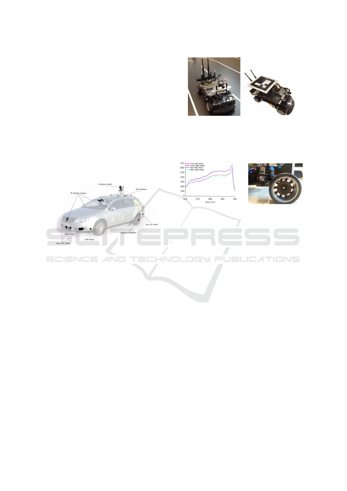
Figure 1: Overview of the Sensor Positioning on MIG au-

tonomous vehicle.

2.2 Autominy TX1

Autominy, shown in Figure 2, is an autonomous

model vehicle based on a scaled 1:10 RC car chas-

sis, with a complete onboard system supplied with

perception sensors, high computing CPU and GPU

power, as well as LEDs to emulate car lights. The car

runs under Ubuntu 18.04 and ROS melodic (Stanford

Artiﬁcial Intelligence Laboratory et al., ). The avail-

able packages allow the car to drive autonomously

and the user to read the Inertial Measurement Unit

(IMU), the wheel velocities, the position of the steer-

ing wheel and the camera images.

Fig. 3a shows a graphic with the measured wheel

velocities while the car is driving in circles. The

mounted sensor is shown in Fig. 3b. We installed a set

of three cameras on the lab ceiling to obtain ground-

truth global localization.

In this work, both the MIG platform and the Au-

tominy were used to develop the localization ap-

proach. The Autominy TX1 is particularly essential

since the wheel odometry network was improved us-

ing the data generated with extreme manoeuvres, and

(a) (b)

Figure 2: Developed (2018) Autominy TX1 version with

odometry research purposes. a) Autominy TX1 on a track

made with black rubber used to achieve aggressive driving

manoeuvres, The ARUCO marker in b) is used to localize

the car on the track.

(a) (b)

Figure 3: A) Wheel Angular Velocities of Autominy TX1.

Front and rear left wheels have a bigger angular velocity

since the car is driving on circles counterclockwise; when

the car stops, velocities drop to zero. b) The Hall sensor

mounted on the car chassis and the magnetic ring installed

on the wheels.

driving manually between the limits of the localiza-

tion set up in the lab.

3 RELATED WORK

The Ackermann approach is derived from the geomet-

rical assumption that the vehicle has a four-bar steer-

ing mechanism and the car moves in perfect circles

which centre I is localized on the rear wheel axis and

in the intersection point of the perpendicular projec-

tions from the pointing wheel direction (see Fig.4).

Moreover, in the models based on Ackermann, the

mathematical approach assumes that the arc on which

the car moves between origins, can be approximated

up to the second-order as ∆ = |O

k+1

|, taking the

following equations to calculate displacement with

Ackermann kinematics derived from Fig.4:

k+1

= x

+ ∆cos(θ

+ ω/2)

k+1

= y

+ ∆sin(θ

+ ω/2)

k+1

= θ

+ ω

(1)

Where x,y and θ are the 2D coordinates of the car

in different k instants of time, ∆ is the travelled dis-

ROBOVIS 2020 - International Conference on Robotics, Computer Vision and Intelligent Systems

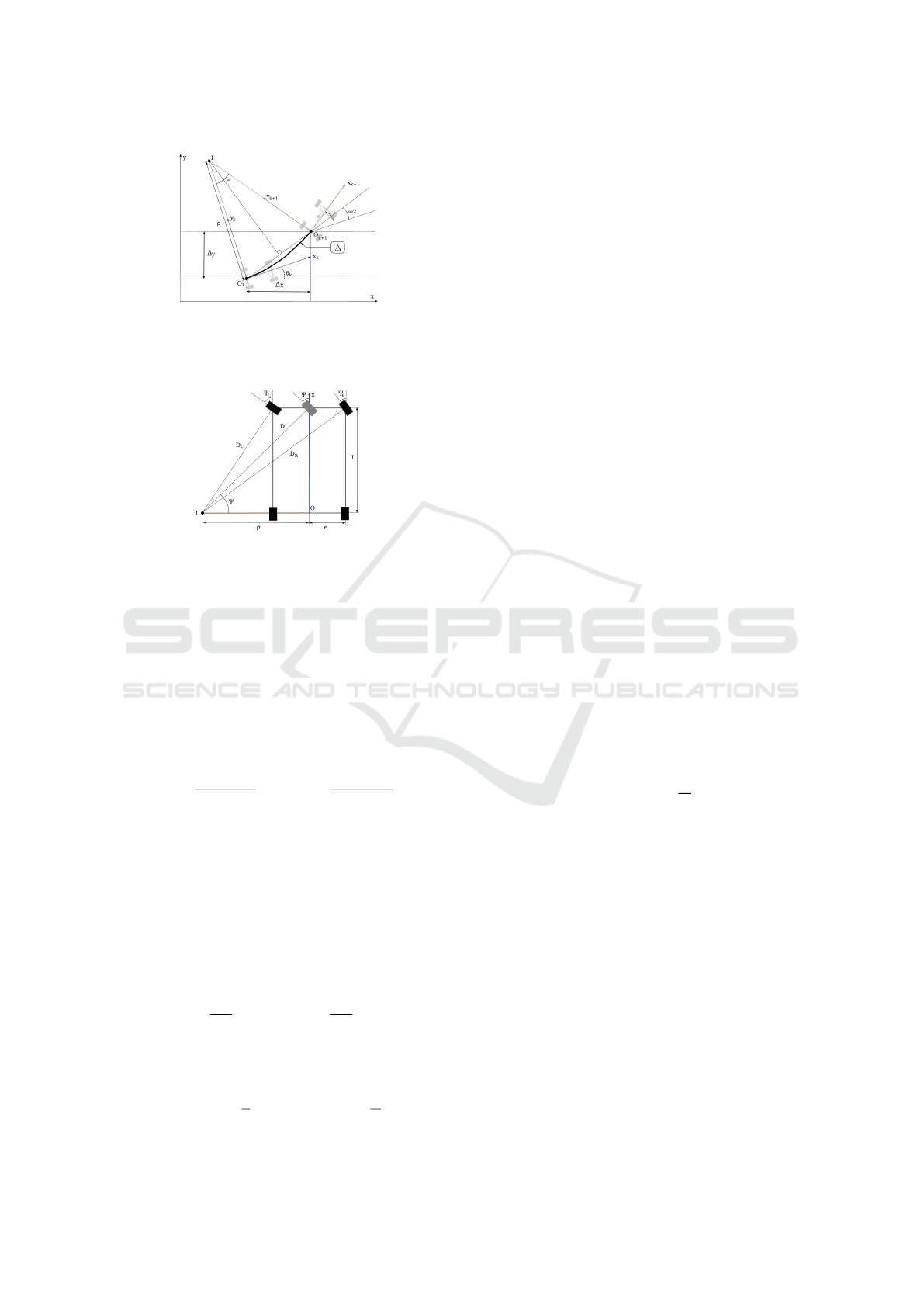
Figure 4: Ackermann steering geometry on a global frame.

I is the instantaneous center of rotation between the car

frames O

and O

k+1

, ∆ is the traveled distance and ρ is the

radius.

Figure 5: Geometry of the car related to the mobile frame O.

Ψ is the Ackermann angle which is referenced on a middle

virtual wheel, ρ is the radius, e is the half track and L the

wheel-base of the vehicle.

tance, and ω is the angle between coordinate systems

of the car on times k and k + 1 related to the instanta-

neous centre of rotation.

In order to calculate ∆ and ω, data obtained from

the ABS should be used. In the most basic approach,

the differential odometry can be calculated from the

rear wheel displacement as follows:

∆ =

+ δ

ω =

− δ

(2)

where δ is the linear displacement of the wheel in

meters, the sub-indexes RR and RL correspond to the

Rear Right wheel and the Rear Left wheel and e is the

half-track of the car.

However, tire slip makes differential odometry not

adequate for practical use. The Ackermann angle ψ is

usually used to improve the results. Add the circle

movement constraint, the radius ρ can be calculated

from Fig. 5 as follows:

ρ =

+ e ρ =

− e (3)

Ackermann angle is then included on the equation

list with the radius or the displacement:

tan(Ψ) =

tan(Ψ) = L

∆

(4)

were L is the wheel-base distance of the car. It

is theoretically possible to compute an Ackermann

odometry using the steering angle sensor of the car to

calculate ω with Eq. (4) and integrating the velocity

measurements of each wheel from the ABS sensors to

calculate ∆ with Eq. (2).

In a vehicle the effective half-track e and the

wheel-base L are not constant due to external distur-

bances like the suspension system, the wheel contact

area with the ﬂoor which modiﬁes the tire force and

wear of the materials. Additionally, in practice, the

Ackermann steering geometry of the mechanism can

be changed to affect the dynamic settings of the car. In

order to measure the Ackermann angle, the Steering

Wheel Angle Sensor (SAS) of the car must be mapped

between the wheel position and the wheel Ackermann

angle.

The relationship between the steering sensor and

the Ackermann angle can be approximated using the

SAS ((Fejes, 2016), (Kallasi et al., 2017)). The ap-

proximation function holds just for a known work-

ing acceleration and velocity threshold, deﬁned by the

user.

Notwithstanding that the mathematical structure

of the Ackermann principle is simple, the tire force

is not taken into account. It is necessary since the

wheels usually do not move on their heading direc-

tion. Therefore, a more precise concept of odometry

must then take into account the Vehicle Slip Angle

(VSA). VSA, also known as the drifting angle, is the

angle between the vehicle longitudinal axis and the

direction of travel, taking the centre of gravity as a

reference ((Chindamo et al., 2018)). The VSA is cal-

culated as follows:

β = −arctan





(5)

where v

and v

are the longitudinal and lateral

velocity of the car. The VSA is widely used for sta-

bility controllers such as ESC (Yim, 2017) or VSC

(Fukada, 1999), AFS (Bechtoff et al., 2016), MPC

(Zanon et al., 2014), among others. Typically for such

applications, an accuracy of 0.1 degrees is needed.

The stability controllers regulate the tracking force of

each wheel employing the brakes in the vehicle. In

this way, it is possible to have a point of rotation I

as close to the perpendicular projection of the centre

of gravity. Therefore, in terms of localization, having

such controllers help to ensure that the vehicle has

a common center of rotation among the four wheels.

With this assumption, a new estimation of the trajec-

tory can be formulated.

To estimate VSA through GPS-inertial sensors,

(Kiencke and Nielsen, 2000) compute the slip angle

GALNet: An End-to-End Deep Neural Network for Ground Localization of Autonomous Cars

employing the bicycle model as follows:

β =

−

ψ (6)

where v

+ v

is the velocity of the vehicle,

ψ is the yaw rate and a

is the lateral acceleration. In

this article, this approximation is used as a character-

istic to train the network.

The ﬁrst efforts to integrate a learning agent to

the estimations fused two methods, an observer (typ-

ically an EKF) which estimates the dynamic of the

car and the neural network estimates the tire data

((Acosta Reche and Kanarachos, 2017), (Dye and

Lankarani, 2016)).

Most of the authors used a general approach of a

three-layered neural network: the input layer, one hid-

den layer and the output layer. The ﬁrst and second

layer use log-sigmoid transfer function and a linear

activation on the last layer ((Wei et al., 2016), (Brod-

erick et al., 2009), (Li et al., 2016)).

Different state inputs to the net were evaluated.

The neural network which was able to estimate a bet-

ter VSA takes into account the change on dynamic

parameters respect to time.

Although the VSA estimator with neural networks

shows sufﬁcient accuracy in practical applications,

the main issues up to today remain in the inability of

the net to adapt after the training if the vehicle param-

eters change and the option to deal with a road bank-

ing angle which has to be estimated with an external

algorithm and then ﬁlter out the lateral acceleration

component due to gravity as in (Sasaki and Nishi-

maki, 2000), and (Melzi et al., 2006). In (Reina et al.,

2010), visual VSA has been used in non-holonomic

robots to correct odometry estimations.

Neural networks and deep learning have shown

their abilities to overcome analytical methods in disci-

plines such as time series forecasting. The application

of neural network methods based on vision in vehi-

cle localization has been widely studied ((Konda and

Memisevic, 2015),(Wang et al., 2017),(Zhan et al.,

2018)). However, very few studies use other sen-

sors such as odometer, imu and GPS. (Brossard and

Bonnabel, 2019) proposed a Gaussian Process com-

bined with neural network and variations inference to

improve the propagation and measurement functions,

thereby improving the localization accuracy. (Belha-

jem et al., 2018) trained a network to learn the lo-

calization error of EKF when GPS was available and

use the network for pose prediction during GPS sig-

nal outage. Different from the existing researches, we

trained an end-to-end neural network to learn the VSA

rate to assist the pose estimation.

4 PROPOSED METHOD

To be able to train a neural network though supervised

learning, we build a dataset that stores an input array

of size nx9 every ∆ of time, being n the number of

timestamps in the dataset. Each row in the matrix has

the following features:

I = [δ,v

re f

,ω

f l

,ω

f r

] (7)

where: δ is the steering angle, v

re f

is the speed

over ground, a

is the longitudinal acceleration, a

the cross acceleration,

is the yaw rate and ω

the speed of the front and rear wheels.

The idea behind including just the variables in

7 and not other parameters such as constant vehicle

mass, size of the wheel-base, wheel diameter or oth-

ers, is that we are looking for a more complex rep-

resentation of these parameters that allow the neural

network to predict odometry for different size of ve-

hicles.

Since an element of the dataset describes the in-

stantaneous dynamic state of the car, we build the in-

puts of the net as a concatenated pair of vectors of 7,

for instance:

= [I

i+1

] (8)

For the net output, we compose an array of size

nx4, which includes the poses of the car. Instead

of recording the global pose, we stored local relative

poses. Local poses allow us to predict local displace-

ments with the net.

To ease the net training, we reduced the problem

to a two-dimensional trajectory. Although for two-

dimensional estimation, only the Yaw angle to deﬁne

orientation is needed, we stored the quaternion values;

during training, the quaternion representation showed

to help the net to converge faster. In an Euler rota-

tion of the format ZY X, the non zero values q

and q

are the last two items of a quaternion. The generated

vector is then as follows:

= [x,y,q

]

One crucial aspect of the data set generation is the

frequency at which the data is sampled. The rate of

the Autominy localization is due to the frame rate

of the ceiling cameras and the post-processing algo-

rithm, which stitch the images, detect the ARUCO

markers, and calculate the position of the car. There-

fore, the sampling rate of the Autominy dataset is

30Hz, while the sampling rate for the MIG dataset

can be conﬁgured up to 100Hz.

In order to avoid redundant data, the reading rate

in the MIG was also conﬁgured to 30Hz; in this way,

ROBOVIS 2020 - International Conference on Robotics, Computer Vision and Intelligent Systems

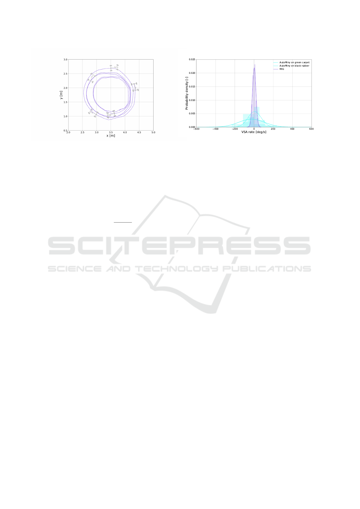
Figure 6: Autominy circle trajectory carried out with the

same steering angle while increasing velocity, which devel-

oped high VSA and VSA rates.

we averaged a travelled distance of 0.5 m per time-

step. We carried out a sanity check before storing the

data. The sanity check veriﬁes that the candidate vec-

tor is not similar to any of the already stored vectors

through cosine similarity, which is a dimensionless

measure for vectors, which are typically sparse.

sim(x,y) =

x · y

kxkkyk

(9)

The similarity equation 9 computes the cosine be-

tween two multidimensional vectors so that a value

of zero means the vectors are perpendicular to each

other, the closer the cosine value to one, the smaller

the angle and the higher the match between vectors.

In our experiments, this value was set to 0.9.

The sanity check also copes with periodic GPS

corrections of the Applanix. Those corrections pro-

duce discrete spatial jumps up to 0.5 m. Since those

jumps in a position generate a non-continuous trajec-

tory, the dataset is sectioned every time a jump is de-

tected. In this way, we store small continuous tra-

jectories with local transformations instead of a long

trajectory with global transformations.

4.1 Dataset Assembling

The datasets were obtained reading the recorded ros-

bags showed in Tables 1 and 2. Autominy was driven

manually in two different trajectories, under variable

dynamic behaviours. Fig. 6 shows a trajectory of the

Autominy periodically increasing its velocity without

changing the steering angle. The vehicle develops

high VSA, which explains the change of the radius

in the spiral trajectory.

Autominy data was recorded using two different

surfaces, Cut Pile green carpet, and PVC black rub-

ber. Driving on different surfaces allowed us to gen-

erate diverse, dynamic performances. While on the

Figure 7: Range of VSA rates (

β) in the datasets. Autominy

developed higher

β over black rubber, while as expected,

the MIG performed the smallest values.

rubber surface, the car was able to drift easily, on car-

pet it was more stable on the curves. Analyzing how

the dynamics of the car changes on such different sur-

faces is key to develop more accurate controllers and

estimators. In this sense, another advantage of using

scaled models is the ease of studying such properties

by changing the surface conditions on the lab ﬂoor.

The dataset of the MIG was recorded in the city

of Berlin on ten different expeditions. There are

no recorded datasets while driving on snow or rain.

Therefore, it is of our interest to expand the dynamic

scope of the MIG trained network by means of in-

cluding the founded associations under the Autominy

dataset.

To examine the dynamic range of the datasets, it is

possible to visualize the slip angle rate derived from

Eq. 5. For Autominy, the Probability Distribution

Function (PDF) of each friction surface is shown in

Fig. 7 together to the MIG slip angle rate, consider-

ing that the available trajectories of the MIG are only

recorded on asphalt, in an average velocity of 20 m/s;

therefore only one PDF of slip angle rate is shown.

As shown in Fig.7, we drove the Autominy on

a higher dynamical range than the MIG. The differ-

ences between the experiments, improve the accuracy

of the MIG net by increasing the gamut of the data

on which the net is trained. The overlapping between

both ranges, allow the net to build a standard feature

map between the Autominy and MIG dynamics.

In Table 1, the amount of train and validation

timestamps are shown. Since on each dataset of Au-

tominy, the trajectories are constantly repeated, the

test section can be safely taken from the same ﬁle and

use it to evaluate the results of the net. In the counter-

part, the MIG rosbags are unique trajectories, and we

are interested in leaving trajectories entirely for test-

ing, owing to the fact that we would like to analyze

how the net generalize for unseen trajectories.

We acknowledge that the partition of the datasets

GALNet: An End-to-End Deep Neural Network for Ground Localization of Autonomous Cars

Table 1: Recorded rosbags in Autominy over black rubber

(br) and green carpet (gc). Different scenarios where used to

increase the range of the dynamic parameters in the vehicle.

#Timestamps Driven

Scenario Train Val. Test length(m)

br driving 2451 817 817 285.7

br drifting 2375 791 791 216.6

gc driving 4716 1578 1578 537.9

gc drifting 3892 1291 1291 349.2

Total 13434 4477 4477 1389.4

Table 2: Recorded rosbags in the MIG and the number of

timestamps in the dataset. Sequences 3, 4 and 8 are used

only for testing, meanwhile the rest of the sequences are

divided between validation and training.

#Timestamps Driven

Scenario Train Val. Test length(m)

FU to OBI 1260 314 0 2356.4

safari online 7326 1831 0 12461.4

thielallee 0 0 3058 4795.3

eng 0 0 583 944.8

react4 1560 389 0 2853.9

reinickendorf 419 104 0 1659.5

aut7 2784 695 0 5907.6

auto8 0 0 1061 1487.9

2tegel 3084 771 0 9968.6

back2fu 1680 419 0 8326.9

Total 18113 4523 4702 50762.3

into training and validation could avert some inter-

esting dynamic information to the net if the data

is indiscriminately divided; therefore, K-fold cross-

validation was used to evaluate the performance of

training on unseen data. The dataset was divided into

four groups (K = 4). To train the ﬁnal model, from

the total timestamps in the Autominy dataset, 60%

were taken for training, 20% for validation and 20%

for testing. In the MIG dataset, seven sequences were

divided between 80% training and 20% validation and

the rest three sequences were used to test.

Each column of the resulting dataset matrix con-

tains the mean and standard deviation of the column

obtained from standardizing the data by subtracting

the mean and dividing by the standard deviation. This

way of representing the data is more convenient for

the training of the net. The complete database is

composed of 22388 samples from the Autominy and

27338 samples from the MIG.

Since the problem is treated as time-series, the

dataset is not shufﬂed randomly. Instead, it is divided

into several sequences of different sizes with differ-

ent starts and endings. This data division expands the

learning dataset, in an analogy to dataset augmenta-

tion for image-learning tasks. The initial member of

each sequence is taken as the initial position of the se-

ries, and the transformations are recalculated. Never-

theless, we trained the net to learn the local transfor-

mations between timestamps. Therefore, to test the

net, it is necessary to estimate the global position of

the vehicle by calculating the SE(3) transformation

to the origin frame. It was found that feeding differ-

ent sequence sizes, and shufﬂing such sequences each

epoch, improved the performance of the net signiﬁ-

cantly. The validation and test datasets are not divided

into smaller sequences, but the full sequences are es-

timated.

We ﬁrst trained the net with the Autominy

database, then, the feature map was used to train the

net for the MIG.

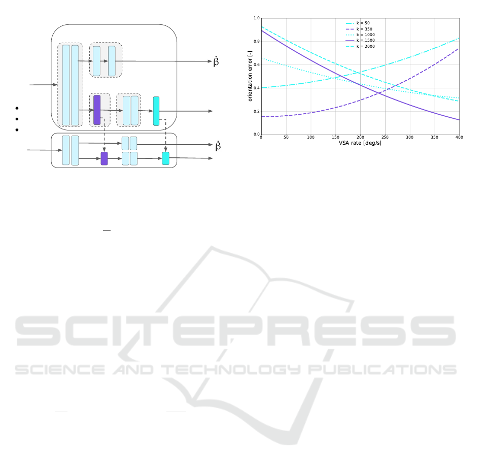
4.2 Architecture Description

The network architecture of our Ground Autonomous

Localization Net (GALNet) is shown in Fig. 8. This

work utilizes Long Short Term Memory (LSTM) with

a projection layer and two regression heads to esti-

mate the slip-slip angle and localization. The LSTM

exploits correlations among the time-correlated data

samples in long trajectories by introducing memory

gates and units (Hochreiter and Schmidhuber, 1997)

in order to decrease the vanishing gradient problem

(Hochreiter, 1998). Although LSTM has the ability to

handle long-term dependencies, learning them is not

trivial. In this work, a series of linear convolutional

layers are used to extract model dynamics.

The net is represented on times k and k + 1 to

show how the states of the LSTM and SO3 layers

are forward propagated to the next training step. The

ﬁrst two fully connected layers compute the ﬁrst re-

lationship between the dynamic variables. We use

this block in the way of an encoder for the derived

two outputs. In one side another dense block com-

putes the VSA rate. The second output is made of an

LSTM layer which ﬁnds the time series relationships,

followed by a fully connected couple of layers that re-

duce the dimensionality to ﬁt the pose output vector.

The net estimates local transformation between two

timestamps. Therefore, a ﬁxed custom layer projects

the displacement to a global frame.

4.3 Loss Functions

The model uses the slip angle as an auxiliary input to

the pose regression. Therefore, there are two losses in

the model. One to predict the correct slip angle and

other to regress the position. The loss regarding slip

ROBOVIS 2020 - International Conference on Robotics, Computer Vision and Intelligent Systems

128

512

k+n

248

128

512

248

LSTM

Fully-

Connecte

Fully-

Connected

Net

output

k+1

SO3

Input

vector

Fully-

Connected

Custom

Layer

Neural Network Architecture

Figure 8: Architecture of GALNet.

angle is as follows:

V SA

∑

−

(10)

where N is the size of the batch.

The proposed method can be considered to com-

pute the conditional probability of the poses Y

,...,y

) given a sequence of vector 7 in time t

p(Y

) = p(y

,...,y

,...,x

)

In order to maximize the previous equation, the

parameters of the net can be found based on Mean

Square Error (MSE). The Euclidean distance between

the ground truth pose y

= (p

,Φ

) and its estimate

= (

) at time k can be minimized by

POS

|N|

∑

− x

+ κ



−



(11)

The factor κ scales the loss between euclidean dis-

tance and orientation error to be approximately equal.

q is in quaternion representation in order to avoid

problems of Euler singularities in the global coordi-

nate frame. Therefore the set of rotations lives on the

unit sphere. During training, the values of

q and q

become close enough to be negligibly compared to

the euclidean distance. Consequently, the constant κ

play an essential role in the accuracy of the net. As a

preliminary setting, we use the approach of (Kendall

et al., 2015) where a constant κ was tuned using grid

search.

Nevertheless, we observed that the error in orien-

tation and position was related not only to κ but also

with VSA rate. Selecting a constant κ value with low

orientation error in small VSA rates (

β), increased the

orientation error on high VSA rates. When a new

value was tested for high

β, the orientation error in-

creased for low VSA rates. Fig.9 shows an iteration

Figure 9: Orientation error for different values of κ related

to the VSA rate (

β). Best values of κ for low and high

β are

showed in purple.

of κ values related to the associated VSA rate. Best

value for almost zero

β was found in κ = 350 while

the best value for the higher rates (400 deg/s) was

found to be around κ = 1500.

This results lead to the idea of a self-tuned κ de-

pending on

β which is as shown on Fig. 8 also pre-

dicted by the net. In order to adapt the scale value, a

Gaussian function is proposed as follows:

κ(

β) = b − ae

−

(

β−µ

)

2σ

(12)

where κ is the loss scale value,

β is the VSA rate.

b shift vertically the function in order to get the min-

imum value of κ when

β is close to zero. a is the

amplitude of the function, σ is the standard deviation

and µ the mean of the normal distribution. σ and µ are

tuned looking for the smaller orientation error with

respect to

β. For the experiments, best values where

found around a = 2300, b = 2000, µ = 0 and σ = 320.

The ﬁnal position regressor layer is randomly ini-

tialized so that the norm of the weights corresponding

to each position dimension was proportional to that

dimension’s spatial extent.

Since the MIG database is more extent in the num-

ber of samples, the ﬁrst net was trained using only

this database. In order to train the Autominy net, the

same architecture was used. To achieve better accu-

racy, the feature map of the previously trained GAL-

Net for MIG was used, the layer group which deter-

mines the dynamic parameters is removed, as well as

the last layer which composes the relative movement.

Finally, the feature map obtained from the second

training is used to ﬁne-tune the MIG net model. This

exploits the associations made by the agent under the

training in the Autominy dataset.

GALNet: An End-to-End Deep Neural Network for Ground Localization of Autonomous Cars

5 EXPERIMENTAL RESULTS

In this section, we brieﬂy summarise the results of the

proposed architecture for dynamic ground localiza-

tion. We employ the Absolute Trajectory Error (ATE)

and Relative Pose Error (RPE) metrics proposed in

(Sturm et al., 2012).

5.1 Evaluation Algorithms

In order to evaluate the proposed model, we compared

the results with two analytical methods.

The ﬁrst algorithm is an Ackermann model odom-

etry which is based on the wheel velocities, and an

estimated Yaw rate obtained from the MIG’s ABS

subsystem. Originally, only the differential velocities

of the back wheels were used in the MIG to deter-

mine the direction and displacement of the car; the

major drawback of the differential odometry was that

the wheel ticks have a systematic error that depends,

among other things, on the wheel pressure, this phys-

ical event provoked the estimated trajectory to drift.

In order to compensate for the deviation, the yaw

rate information from MIG’s ABS subsystem was in-

volved. For the results section of this article, we iden-

tify this Ackermann-compensated differential odom-

etry as WO.

The second algorithm is a self-implemented Un-

scented Kalman ﬁlter (UKF) estimator which inte-

grates the WO and IMU measurements from the car

inertial unit. The ﬁlter is obtained employing the

ROS robot-localization package (Moore and Stouch,

2014).

The net was ﬁrst trained on the MIG dataset, and

the feature map was then used to train the net with the

Autominy dataset. We differentiate the networks in

the evaluation as GALNet and iGALNet correspond-

ingly.

5.2 Quantitative Evaluation of

Trajectories

In order to measure the errors on the ﬁnal trained neu-

ral network, Table 3 shows the performance of the net

with the ATE metric and Table 4 shows the RPE for

the MIG trajectories.

Table 3 shows that in some trajectories GALNet

and iGALNet improve the baseline methods. It is in-

teresting to notice that not in all cases iGALNet per-

forms better than GALNet, which means some asso-

ciations are lost in the over-training process.

Table 4 shows that for the MIG, local displace-

ments are still better estimated with WO. This result

is expected since most of the short trajectories that

Table 3: ATE translational error in meters of the MIG

dataset before and after including the Autominy dataset in

the training. The methods used to compare are: MIG Wheel

Odometry (WO), Unscented Kalman Filter (UKF), GAL-

Net trained only with the MIG dataset, and the improved

version (IGALNet) trained with the Autominy dataset.

Method Wo UKF GALNet iGALNet

FU to OBI 86.87 42.51 88.48 43.43

safari online 428.31 4.60 483.21 50.00

thielallee 55.97 13.84 199.5 11.87

englerallee 132.07 167.5 9.20 46.61

react4 24.33 19.10 67.65 10.39

reinickendorf 6.47 3.65 2.84 2.46

auto7 211.96 17.97 89.86 12.36

auto8 17.35 3.73 46.73 4.62

tegel 269.55 4.48 219.55 23.72

back2fu 506.92 7.15 126.48 18.33

Table 4: RPE translational error in meters of the MIG

dataset before and after including the Autominy dataset in

the training. The methods used to compare are: Mig wheel

Odometry (WO), Unscented Kalman Filter (UKF), GAL-

Net trained only with the MIG dataset and the improved

version (iGALNet) trained with the Autominy dataset.

Method Wo UKF GALNet iGALNet

FU to OBI 0.43 0.49 0.71 0.59

safari online 0.27 0.28 1.26 0.45

thielallee 0.41 0.51 0.79 0.60

englerallee 0.44 0.58 0.77 0.74

react4 0.43 0.49 0.70 0.55

reinickendorf 0.51 0.63 0.70 0.65

auto7 0.39 0.48 0.89 0.60

auto8 0.31 0.28 0.42 0.27

tegel 0.95 1.09 1.49 1.34

back2fu 2.77 3.09 4.04 3.13

are sampled at 30 Hz and have a mean displacement

of 0.5 m are straight trajectories. Therefore, integra-

tion of the angular wheel velocity is still a better ap-

proximation for straight driving. WO has its major

disadvantage on estimating orientation. In a global

trajectory, orientation errors are collaterally translated

to translational errors. For that reason, wheel odom-

etry performs worse with the ATE metric. For some

datasets, the precision of the UKF is achieved with

the proposed methods.

Because the net was trained to estimate displace-

ment between two consecutive relative positions, it is

interesting to examine the RPE metric deeper and ob-

serve how the error develops since the GPS adjust-

ments are represented as outliers. For this analysis,

we selected the Safari trajectory. Fig. 10 and 11 show

the RPE violin histograms of the translational and ro-

tational components of the relative transformations.

Fig. 10 corroborates the values in Tab. 3, where

ROBOVIS 2020 - International Conference on Robotics, Computer Vision and Intelligent Systems

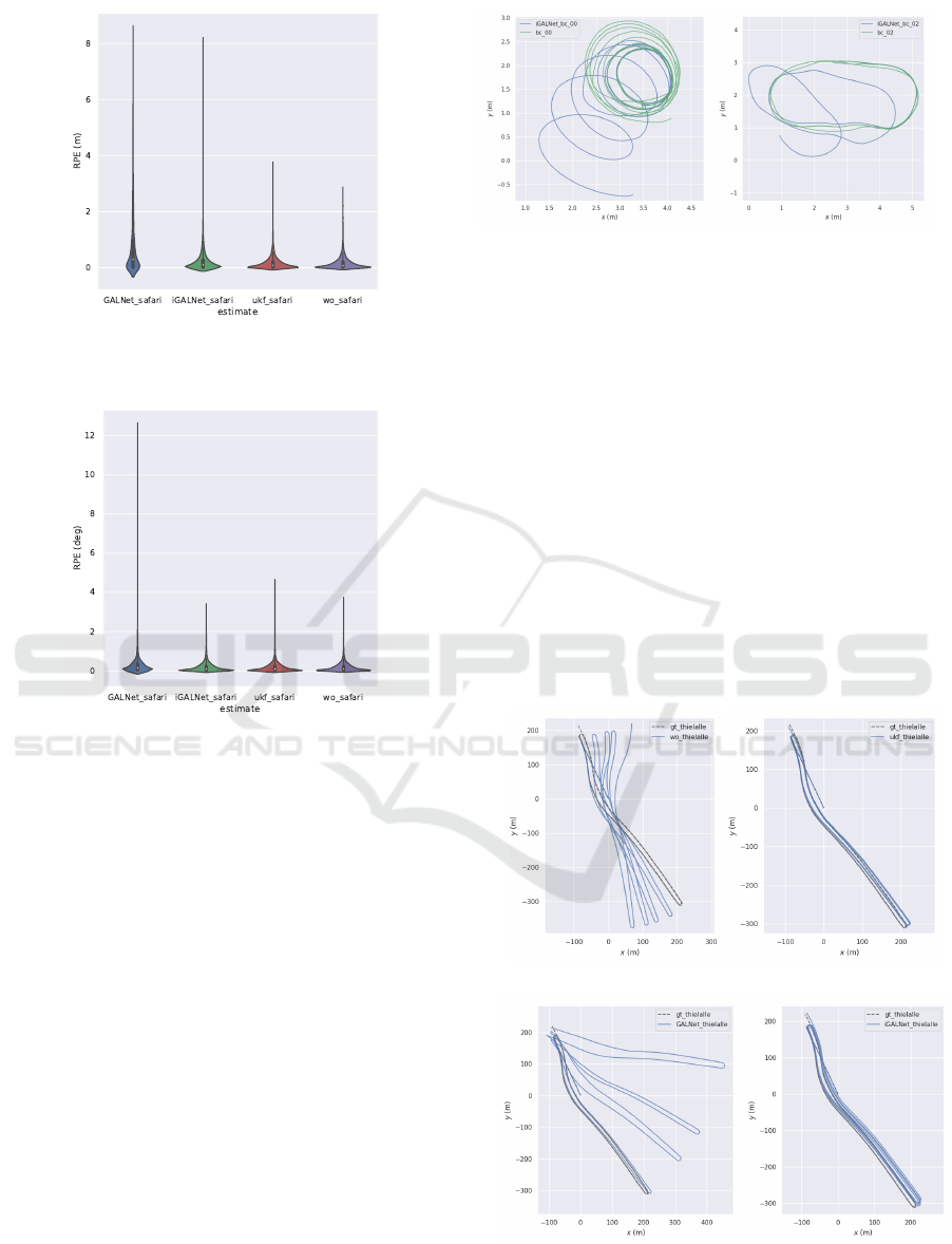
Figure 10: RPE violin histogram of the translational errors

in meters in the Safari trajectory.

Figure 11: RPE violin histogram of the rotational errors in

degrees in the Safari trajectory.

the WO estimates more effectively the translational

displacement, while its biggest error is around 3 m

the iGALNet goes up to 9 m, the errors accumulate

closer to zero than the other algorithms. It also shows

the improvement of iGALNet against GALNet. Even

that the purpose of training on the Autominy dataset

was to reduce rotational error focusing on VSA, trans-

lational error improved as well. However, this re-

sult suggests that a pure translational displacement

dataset, generated with the Autominy could help the

estimation.

In Fig. 11, the reduction of outliers between GAL-

Net and iGALNet is more evident. The proposed deep

neural network has a better rotational performance

than the evaluation algorithms, which was the purpose

of this work. The iGALNet network has the smallest

outliers and its error distribution closer to zero than

the rest of the algorithms.

The resemblance between the violin distributions

of the different algorithms shows that the proposed

neural network was able to ﬁnd the correct associa-

tions to estimate composed displacement.

(a) (b)

Figure 12: A) Seq. 00 of the Autominy dataset, transla-

tional errors are: ATE=1.37 RPE=0.03. b) Seq. 02 of

the Autominy dataset, translational errors are: ATE=2.16

RPE=0.01. On the green the ground truth obtained with the

ceiling cameras in the lab, in blue, the estimated trajectory

of iGALNet.

5.3 Qualitative Evaluation of

Trajectories

Although the net was able to improve for small

and therefore contribute to the precision in the MIG

dataset, the high rates in the Autominy dataset showed

limited precision. Fig. 12 shows two trajectories

driven in the lab with Autominy where

β values went

up to 1.2 rad/s.

Figure 13 shows the trajectories of the MIG wheel

odometry, UKF and GALNet before and after (iGAL-

(a) (b)

Figure 13: Resulting trajectories of the proposed methods in

Thielallee. a) MIG wheel odometry, b) UKF wheel-inertial

odometry, c) GALNet, d) iGALNet.

GALNet: An End-to-End Deep Neural Network for Ground Localization of Autonomous Cars

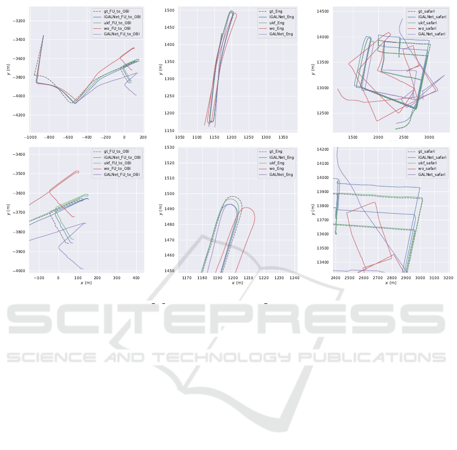
Figure 14: Trajectories in datasets FU to OBI, Englerallee and safari online, showing complete and close up of them.

Net) being trained with the Autominy dataset in

Thielallee, the ofﬁcial test area of the MIG in Berlin.

Fig. 14 - 16 show the rest of the resulting trajectories

in the MIG dataset, which give a more visual evalua-

tion of them.

5.4 Reported Runtime

The network is implemented based on the TensorFlow

framework and trained using an NVIDIA Geforce

RTX 2080 ti. Adam optimizer is employed to train

the network with starting learning rate 0.001 and pa-

rameters α

= 0.9 and α

= 0.999 both values recom-

mended on the analysis in (Kingma and Ba, 2014).

The training was set for 200 epochs but using call-

back Tensorﬂow implementations such as early stop-

ping if the loss function does not decrease 0.001 for

more than ﬁve epochs to reduce the training time.

Training time on all the trajectories takes approx-

imately 10k to 50k iterations or 2 hours to 6 hours.

Prediction time for an input vector pair takes on aver-

age 25 ms, i.e., 40Hz.

6 CONCLUSIONS

We introduced GALNet, a deep learning architecture

for pose estimation employing inertial, kinematic, and

wheel velocity data from the car. We employed VSA

rate as the main characteristic to estimate vehicle dis-

placements.

We showed that it is possible to use the experi-

ments performed by different vehicles to improve the

results of the deep neural network model. The re-

sults of the estimation were compared with a Classical

Unscented Kalman Filter predictor and a basic wheel

odometry scheme. Transferring learning between two

different experimental platforms brings advantages to

the accuracy of the net. However, the model is highly

dependent on the sensor, which provides ground truth,

and the intrinsic drifting of the device is also trans-

ferred to the model.

The proposed method shows that, with enough in-

formation, a robust net can be trained. The perfor-

mance of the net is information-dependent. If the

characteristics of the dynamic system changes, the es-

timated position could be improved with more data

collection. Therefore the system could be reﬁned on-

line on a test vehicle and update the weights of the net

to avoid wide drifting errors.

ROBOVIS 2020 - International Conference on Robotics, Computer Vision and Intelligent Systems

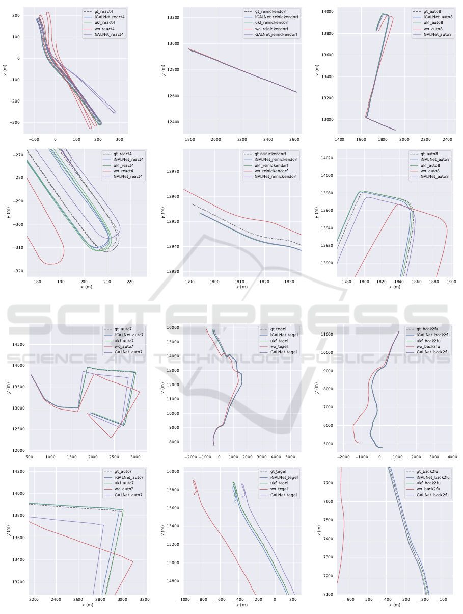
Figure 15: Trajectories in datasets react4, reinickendorf and auto8.

Figure 16: Trajectories in datasets auto7, tegel and back2fu.

GALNet: An End-to-End Deep Neural Network for Ground Localization of Autonomous Cars

We showed that it is possible to increment the ac-

curacy of the models by complementing the dataset.

Implementing a model that can integrate more infor-

mation to improve the learning process during driving

is a direction for future work.

REFERENCES

Acosta Reche, M. and Kanarachos, S. (2017). Tire lateral

force estimation and grip potential identiﬁcation using

neural networks, extended kalman ﬁlter, and recursive

least squares. Neural Computing and Applications,

2017:1–21.

Bechtoff, J., Koenig, L., and Isermann, R. (2016).

Cornering stiffness and sideslip angle estimation

for integrated vehicle dynamics control. IFAC-

PapersOnLine, 49(11):297 – 304. 8th IFAC Sympo-

sium on Advances in Automotive Control AAC 2016.

Belhajem, I., Maissa, Y. B., and Tamtaoui, A. (2018).

Improving low cost sensor based vehicle positioning

with machine learning. Control Engineering Practice,

74:168–176.

Broderick, D., Bevly, D., and Hung, J. (2009). An adaptive

non-linear state estimator for vehicle lateral dynamics.

pages 1450–1455.

Brossard, M. and Bonnabel, S. (2019). Learning wheel

odometry and imu errors for localization. In 2019 In-

ternational Conference on Robotics and Automation

(ICRA), pages 291–297. IEEE.

Chindamo, D., Lenzo, B., and Gadola, M. (2018). On the

vehicle sideslip angle estimation: A literature review

of methods, models, and innovations. Applied Sci-

ences, 8(3).

Dye, J. and Lankarani, H. (2016). Hybrid simulation of

a dynamic multibody vehicle suspension system us-

ing neural network modeling ﬁt of tire data. page

V006T09A036.

Fejes, P. (2016). Estimation of steering wheel angle in

heavy-duty trucks.

Fukada, Y. (1999). Slip-angle estimation for vehicle stabil-

ity control. Vehicle System Dynamics, 32(4-5):375–

388.

Hochreiter, S. (1998). The vanishing gradient problem dur-

ing learning recurrent neural nets and problem solu-

tions. International Journal of Uncertainty, Fuzziness

and Knowledge-Based Systems, 6:107–116.

Hochreiter, S. and Schmidhuber, J. (1997). Long short-term

memory. Neural computation, 9:1735–80.

Kallasi, F., Rizzini, D. L., Oleari, F., Magnani, M., and

Caselli, S. (2017). A novel calibration method for

industrial agvs. Robotics and Autonomous Systems,

94:75 – 88.

Kendall, A., Grimes, M., and Cipolla, R. (2015). Convolu-

tional networks for real-time 6-dof camera relocaliza-

tion. CoRR, abs/1505.07427.

Kiencke, U. and Nielsen, L. (2000). Automotive control

systems: For engine, driveline, and vehicle. Measure-

ment Science and Technology, 11(12):1828–1828.

Kingma, D. P. and Ba, J. (2014). Adam: A method for

stochastic optimization.

Konda, K. R. and Memisevic, R. (2015). Learning visual

odometry with a convolutional network. In VISAPP

(1), pages 486–490.

Li, Z., Wang, Y., and Liu, Z. (2016). Unscented kalman

ﬁlter-trained neural networks for slip model predic-

tion. PloS one, 11:e0158492.

Melzi, S., Sabbioni, E., Concas, A., and Pesce, M. (2006).

Vehicle sideslip angle estimation through neural net-

works: Application to experimental data.

Moore, T. and Stouch, D. (2014). A generalized extended

kalman ﬁlter implementation for the robot operating

system. In Proceedings of the 13th International Con-

ference on Intelligent Autonomous Systems (IAS-13).

Springer.

Reina, G., Ishigami, G., Nagatani, K., and Yoshida, K.

(2010). Odometry correction using visual slip angle

estimation for planetary exploration rovers. Advanced

Robotics, 24:359–385.

Sasaki, H. and Nishimaki, T. (2000). A side-slip angle es-

timation using neural network for a wheeled vehicle.

SAE Transactions, 109:1026–1031.

Stanford Artiﬁcial Intelligence Laboratory et al. Robotic

operating system.

Sturm, J., Engelhard, N., Endres, F., Burgard, W., and Cre-

mers, D. (2012). A benchmark for the evaluation of

rgb-d slam systems. pages 573–580.

Valente, M., Joly, C., and de La Fortelle, A. (2019). Deep

sensor fusion for real-time odometry estimation.

Wang, S., Clark, R., Wen, H., and Trigoni, N. (2017).

Deepvo: Towards end-to-end visual odometry with

deep recurrent convolutional neural networks. In 2017

IEEE International Conference on Robotics and Au-

tomation (ICRA), pages 2043–2050.

Wei, W., Shaoyi, B., Lanchun, Z., Kai, Z., Yongzhi, W., and

Weixing, H. (2016). Vehicle sideslip angle estimation

based on general regression neural network. Mathe-

matical Problems in Engineering, 2016:1–7.

Weinstein, A. and Moore, K. (2010). Pose estimation of

ackerman steering vehicles for outdoors autonomous

navigation. pages 579 – 584.

Yim, S. (2017). Coordinated control of esc and afs with

adaptive algorithms. International Journal of Auto-

motive Technology, 18(2):271–277.

Zanon, M., Frasch, J., Vukov, M., Sager, S., and Diehl, M.

(2014). Model Predictive Control of Autonomous Ve-

hicles, volume 455.

Zhan, H., Garg, R., Saroj Weerasekera, C., Li, K., Agar-

wal, H., and Reid, I. (2018). Unsupervised learning

of monocular depth estimation and visual odometry

with deep feature reconstruction. In Proceedings of

the IEEE Conference on Computer Vision and Pattern

Recognition, pages 340–349.

ROBOVIS 2020 - International Conference on Robotics, Computer Vision and Intelligent Systems