Analysis of Free Time Intervals between Buyers at Cash Register using
Generating Functions
Detlef Hartleb
1,2
, Andreas Ahrens
1
, Ojaras Purvinis
3
and Jelena Zaˇsˇcerinska
1,4
1
Hochschule Wismar, University of Technology, Business and Design, Wismar, Germany
2
ETSIST, Universidad Polit´ecnica de Madrid, Madrid, Spain
3
Kaunas University of Technology, Kaunas, Lithuania
4
Centre for Education and Innovation Research, Riga, Latvia
Keywords:
Bottleneck, Buyers’ Burstiness, Cashiers’ Bottleneck, Cash Register, Buyers’ Waiting Time Gaps, Generating
Functions.
Abstract:
The optimization of bursty business processes requires stochastic models with measurable parameters. Often
simplifications worked out in the analysis of such models lead to inaccuracies when events occur in a bursty
manner. In this work, a novel approach based on generating functions is introduced for modelling the bursty
appearance of buyers via gap processes when paying at the cash register. The obtained approach is verified by
analysing the payment process at the cash register by taking the free time intervals (gaps) between buyers as
well as the payment processing time at the cash register into account. As both payment-related processes can
be described by gap processes, the use of generating functions allows close-form solutions when analysing the
payment process at the cash register. As an example the payment process is analysed in two supermarket of
different sizes in Lithuania. The obtained results show that the free time intervals at the cash register are quite
bursty independent of the size of the shop whereas the payment processing intervals at the cash register are
quite regularly distributed.
1 INTRODUCTION
In order to model bursty business systems accurately
when optimizing the performance of such systems
using e. g. the well-known queuing theory, stochas-
tic processes with measurable parameters have to be
found. Such optimizations based on gap-processes
have been studied successfully when analyzing bit-
errors in telecommunication systems (e.g. wireless
systems) (Wilhelm, 1976; Wilhelm, 2018) as well
as packet arrivals in Ethernet-based data networks
(Kessler et al., 2003) or when analyzing the internet
traffic (Kresch and Kulkarni, 2011; Zukerman et al.,
2003), where data packets arrive in bursts as well.
However the concept of gap processes has never been
applied to model the payment process as carried out
in this work.
Bursts correspond to an enhanced activity level
over a short period of time followed by long periods
of inactivity and often leads to bottlenecks. In busi-
ness systems, bottlenecks limit the flow of customers,
services or products, etc. It happens when single busi-
ness processes within the business system operate at
their capacity limit or beyond. Given the diversity of
systems in which burstiness emerges, the modelling
of burstiness plays an important role as bottlenecks
are still an indicator for customers dissatisfaction.
Burstiness in shop sales, as studied in this work,
can be addressed when the components have a mea-
surable activity pattern (such as to buy or not to buy).
Fig. 1 illustrates the customer behaviour in shop sales.
When analyzing the buying process chain, the cus-
tomer arrival at the shop, the selection of goods, the
payment process as well as the customer or buyer de-
parture is meant. In this work a customer is a person
who visits the shop but does not buy anything.
This work is aiming to achieving customer quality
improvement through prevention of queuing by ana-
lyzing the payment process at the cash register (Mice-
viciene et al., 2018; Mittal and Kamakura, 2001; Ku-
mar et al., 2016). The payment process itself can be
divided into the process of buyers’ waiting to the cash
register described by free time intervals between buy-
ers as well as the payment processing time (also re-
ferred as buyers’ service time). Fig. 2 highlights the
two parametersinfluencingthe paymentprocess at the
42
Hartleb, D., Ahrens, A., Purvinis, O. and Zaš
ˇ
cerinska, J.
Analysis of Free Time Intervals between Buyers at Cash Register using Generating Functions.
DOI: 10.5220/0010172700420049
In Proceedings of the 10th International Conference on Pervasive and Parallel Computing, Communication and Sensors (PECCS 2020), pages 42-49
ISBN: 978-989-758-477-0
Copyright
c
 2020 by SCITEPRESS – Science and Technology Publications, Lda. All rights reserved

not to buy
customer arrival
buyer departure
cash register
customer
in the shop
(to buy/not to buy)
shop entrance
to buy
customer flow
through
the shop
customer departure
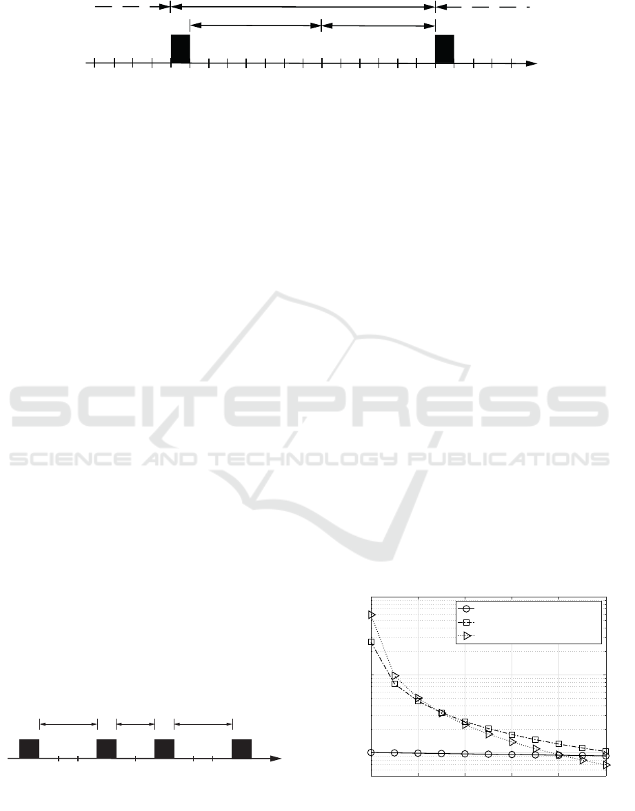
Figure 1: Customer behaviour in shop sales.
cash register. As the payment processing time is usu-
ally determined by technological limits (scanning of
the purchased goods, the paying process itself) and
the experience of the sales staff, only the free time
intervals between buyers to the cash register as an in-
dicator of bottlenecks throughout the whole process
of buying are studied in this work.
The free time intervals between buyers to the cash
register, as indicated in Fig. 3, as well as the payment
processing time intervals are described and modelled
by gaps. The gaps are characterized by the gap distri-
bution function u(k), defined as the probability that a
gap Y between two buyers is greater than or at least
equal to a given number of non-buying customers k,
i. e.
u(k) = P(Y ≥ k) . (1)
Alternatively, the gap-density function v(k) = P(Y =
k) can be used as well, denoting the probability, that
a gap Y of length k appears.
By describing the process of buyers’ waiting to the
cash register and the process of payment individually
by gaps, the payment process can be modelled by two
independent gap-processes with different parameters
as highlighted in Fig. 4. As the payment processing
times are quite regularly distributed, the focus in this
work is put on the free-time intervals between buyers
buyers‘ service
time
free time intervals
(gaps)
between buyers
cash register
capacity utilization
Figure 2: Parameters influencing cash register capacity uti-
lization.
- x - - x - - x - - - x x - - - - x -
2 2 3 40
Figure 3: Modelling free-time intervals between buyers to
the cash register (a buyer (represented by ”x”) within a se-
quence of non-buying customers (represented by ”-”)).
to the cash register.
Often the performance has been studied under
the assumption that the gaps are exponentially dis-
tributed. However, under bursty conditions such ex-
ponential gap distribution functions (Weisstein, 1999)
become inaccurate (Feldmann, 2000; Kessler et al.,
2003; Ahrens et al., 2019b). Thus, for modelling
bursty behaviour, the gap distribution function should
be different from the exponential one. Against this
background, in this work a novel approach for mod-
elling bursty as well as non-bursty business processes
by using generating functions, which will be used to
describe the payment process, is presented.
The concept of generating functions is well-
developed in the research community (Chattamvelli
and Shanmugam, 2019). Generating functions have
been identified as an extremely beneficial tool when
analyzing discrete sequences of infinite length (Zhang
et al., 2016; Li, 1992). Instead of analyzing a se-
quence of infinite length, a single function can be
derived, representing the sequence of infinite length.
For example, the gap-distribution sequence u(k) =
(1,1,1,1, ...) can be represented by the power series
U(t) =
∞
∑
k=0
u(k)t
k
= 1+t + t
2
+ . .. . (2)
This power series converges for |t| < 1 to
U(t) =
∞
∑
k=0
u(k)t
k
=
1
1− t
. (3)
The function U(t), defined in (3), provides an alter-
native description for the gap distribution function
u(k) = (1,1, 1,1,.. .) of infinite length. The elements
of the sequence u(k) are the coefficients of the in-
finite polynomial defined by (2). Such closed form
solutions are known for exponential gap distribution
functions. However,it is ratherdifficultto find closed-
form solutions for gap distribution function that are
different from the exponential one (Wilhelm, 1976;
Wilhelm, 2018).
The novelty of this paperis givenby the use of gen-
erating functions applied to the system model, namely
free time intervals between buyers at the cash register,
for simulating bursty buyers’ behaviour. As an illus-
trative example the free time intervals between buyers
at the cash register are studied in two supermarkets
of different sizes in Lithuania.
Analysis of Free Time Intervals between Buyers at Cash Register using Generating Functions
43

time (in sec)
m
th
-buyer‘s
payment process
(m+1)
th
-buyer‘s
payment process
(m-1)
th
-buyer‘s
payment process
gap process I
(waiting time to cash register)
gap process II
(payment processing time)
Figure 4: Modelling the payment process by two independent gap processes.
The remaining part of this paper is organized as
follows: Section 2 introduces the theoretical basis for
modelling buyers’ behaviour. Section 3 briefly re-
views the basics of using generating functions fol-
lowed by approaches to model bursty as well as non-
bursty buyers’ behaviour. Section 4 is dedicated to the
use of generating functions for gap modelling to anal-
yse bursty as well as non-bursty buyers’ behaviour.
The associated results of an empirical study of differ-
ent grocery shops in Lithuania are discussed in Sec-
tion 5. Finally, some concluding remarksare provided
in Section 6.
2 BURSTY BUSINESS
PROCESSES
Bottlenecks in supermarkets, created by bursty cus-
tomers (i. e. buyers), can limit the capacity of the
whole shop since e. g. more buyers appear at the
cash register than can be served. Conventionally, bot-
tlenecks can be measured by indicators or parame-
ters such as the buyers’ probability and buyers’ con-
centration. These parameters can be obtained when
analysing the gaps between the buyers, i. e. the free
time intervals between the buyers to the cash register
as shown in Fig. 3. Here, stochastic processes with
measurable parameters are needed when analysing
the free time intervals between buyers.
Practically, when analysing the free time inter-
vals between buyers at the cash register as depicted
in Fig. 5, the gap distribution function u(k) can be de-
rived by introducing a suitable time interval t
A
and
discretising the free time intervals t
ℓ
. After mapping
them to the discrete parameter t
ℓ
/t
A
, the subsequent
rounding delivers the discrete gap parameter k
ℓ
.
t
1
t
2
t
3
time
Figure 5: Free time intervals at the cash register.
Alternatively, the gap density function v(k), de-
fined as the probability that a gap Y between two buy-
ers to the cash register is equal to a given number of
non-buying visitors k, is of high interest, too. Taking
the gap density functionv(k) = P(Y = k) into account,
(1) can be re-written as
u(k) = v(k) + v(k+ 1) + v(k + 2) + .. . . (4)
Fig. 6 shows different gap density functions v(k)
when analysing the free time intervals (gaps) between
buyers to the cash register at buyer probability of
p
e
= 10
−2
. With an increasing level of burstiness
as demonstrated in Fig. 6, the probability that after
a buyer in the distance k = 0 another buyer appears,
i. e. v(0), increases. In this situation, the buyers ap-
pear more and more concentrated.
Intuitively, the buyers’ behaviour can be described
by a probability of purchase or buyer probability p
e
(as a percentage of the visitors in the shop who buy
something). However, the buyer probability does
not give any indication of how concentrated the buy-
ers are. In this case the model has to be extended
by at least a second parameter as shown by Wil-
helm (Wilhelm, 1976; Wilhelm, 2018) and Ahrens
(Ahrens et al., 2019a) by introducing buyer concen-
tration (1− α).
A process will appear bursty if the probability of
short gaps is higher and lower for longer gaps if com-
pared with a process with no burstiness (Fig. 6). This
results in many short intervals (gaps) of high activity
(probability) separated by longer intervals (gaps) of
0 2 4 6 8 10
10
-2
10
-1
10
0
no burstiness
medium-level of burstiness
high-level of burstiness
v(k) →
k →
Figure 6: Gap density functions v(k) for different levels of
burstiness at buyer probability of p
e
= 10
−2
.
PECCS 2020 - 10th International Conference on Pervasive and Parallel Computing, Communication and Sensors
44

inactivity.
As shown in (Wilhelm, 1976) and (Ahrens, 2000;
Ahrens et al., 2019a) a good gap distribution function
for bursty as well as non-bursty buyers’ behaviour is
given by
u(k) = [(k + 1)
α
− k
α
] · e
−β·k
. (5)
depending on the buyer probability p
e
and the buyer
concentration (1− α). The parameter β defined in (5)
has to fulfil the following equation
p
e
≈ β
α
(6)
as shown by (Wilhelm, 1976; Wilhelm, 2018). Prac-
tically, relevant buyer concentration is in the range of
0.0 < (1− α) ≤ 0.5, whereas the buyer concentration
of (1− α) = 0 describes the situation with non-bursty
buyers (also refers to memoryless buyer scenario),
where the buyer probability is sufficient to describe
the buying process.
Unfortunately, no generating function for the gap
distribution function u(k), defined in (5), can be de-
rived (Wilhelm, 1976; Wilhelm, 2018), except for
(1− α) = 0.
3 GENERATING FUNCTIONS
Generating functionscan be used for describing an in-
finite sequence of numbers by treating them as the co-
efficients of a power series (Zhang et al., 2016). The
concept of generating functions is well-established in
the research community and used in this work for
modelling the free time intervals (gaps) between buy-
ers at the cash register.
Bursty as well as non-burstyfree time intervals be-
tween buyers to the cash register is described by the
gap distribution function u(k) defined in (1). The gen-
erating function associated to (1) is the power series
U(t) =
∞
∑
k=0
u(k)t
k
. (7)
In the following sections, close-form solutions are de-
rived for both non-bursty as well as bursty free time
intervals between buyers at the cash register.
3.1 Non-bursty Buyers Behaviour to the
Cash Register
For situations with independent events, i. e. buyers
to the cash register, the gap distribution function u(k)
can be defined by the buyers probability p
e
solely as
shown in (Ahrens et al., 2019b) and results in
u(k) = (1 − p
e
)
k
. (8)
Consequently, the generating function is obtained as
U(t) =
∞
∑
k=0
u(k)t
k
=
∞
∑
k=0
(1− p
e
)
k
t
k
. (9)
The generating function is a geometric series with the
quotient q = (1− p
e
)t and leads for |q| < 1 to
U(t) =
∞
∑
k=0
q
k
=
1
1− q
=
1
1− (1− p
e
) · t
. (10)
With the approximation 1 − p
e
≈ e
−p
e
for small p
e
,
the generating function can be re-formulated as
U(t) =
1
1− e
−p
e
·t
. (11)
Given the generating function U(t) defined in (11)
the corresponding elements of the sequence u(k) can
be calculated based on Taylor’s theorem by the k-th
derivative of the generating functionU(t) at the posi-
tion t = 0. The elements of the sequence u(k) result
in
u(k) =
U
k
(0)
k!
(12)
Differentiating the generating function U(t), defined
in (11), the elementsof the series u(k) can be obtained
as
u(0) = 1
u(1) = e
−p
e
≈ (1− p
e
)
u(2) = e
−p
e
· e
−p
e
≈ (1− p
e
)
2
.
.
. =
.
.
.
and confirm (8). The validation of the generating
function can be carried out when analysing the aver-
age gap length (free time intervals) between two buy-
ers to the cash register. Having completely indepen-
dent buyers, the average gap length between two buy-
ers can be expressed by the buyer probability p
e
as
1
p
e
− 1 =
∞
∑
k=0
k· v(k) . (13)
With
∞
∑
k=0
k· v(k) =
∞
∑
k=0
u(k) − 1 (14)
we get
1
p
e
=
∞
∑
k=0
u(k) =
∞
∑
k=0
u(k) · 1
k
. (15)
This equation can be re-written as
1
p
e
=
∞
∑
k=0
u(k) · 1
k
= U(1) (16)
Analysis of Free Time Intervals between Buyers at Cash Register using Generating Functions
45

and is confirmed by U(1) as U(1) results with (11) in
U(1) =
1
1− e
−p
e
≈
1
p
e
. (17)
Therefore, the generating function should be suit-
able for describingnon-bursty buyers behaviour to the
cash register.
3.2 Bursty Buyers Behaviour
For bursty free time intervals between buyers to the
cash register, the following gap distribution function
is identified to be useful
u(k) = [(k + 1)
α
− k
α
] · e
−β·k
, (18)
with the parameter (1 − α) describing the buyer con-
centration and p
e
= β
α
defined as buyer probabil-
ity (Wilhelm, 2018; Ahrens et al., 2019a). Unfor-
tunately, there is no known closed-form solutions
for the corresponding generating function (Wilhelm,
1976). Therefore an approximation for u(k) defined
in (18) has to be applied (Wilhelm, 1976; Wilhelm,
2018). Taking the series expansion of the expression
(k+ ∆k)
α
= k
α
(1+
α
k
∆k + ...) (19)
into account, the expression (18) simplifies with ∆k =
1 to
u(k) ≈
∞
∑
k=0
αk
α−1
e
−β·k
. (20)
Using the integral instead of the sum, the generating
function U(t) results in
U(t) = cα
∞
Z
k=0
k
α−1
e
−β·k
t
k
dk (21)
and can be re-defined as
U(t) = cα
∞
Z
0
k
α−1
e
(ln(t)−β)k
dk . (22)
The parameter c has to be determined in order to fulfil
the condition u(0) = 1. Using the integral
∞
Z
0
k
δ−1
e
−ωk
dk =
Γ(δ)
ω
δ
. (23)
the following solution with ω = β − ln(t) and δ = α
can be obtained
U(t) = cα Γ(α) ·
1
(β− ln(t))
α
, (24)
with the parameter Γ(·) describing the Gamma func-
tion. With
β− ln(t) = (1− (1− [β − ln(t)])) (25)
the expression β − ln(t) can be represented for |β −
ln(t)| ≪ 1 as
β− ln(t) ≈ 1− e
−(β−ln(t))
= 1− e
−β
t (26)
and the generating functionU(t) results in
U(t) = cα Γ(α) ·
1
(1− e
−β
t)
α
(27)
In order to calculate the parameter c, the function
U(t) = u(0)t
0
+ u(1)t
1
+ u(2)t
2
+ · ·· , (28)
has to fulfil the condition
u(0) = 1 → U(0) = 1 , (29)
and therefore the parameter c has to be set
cαΓ(α) = 1 . (30)
Finally, the generating functionU(t) results in
U(t) =
1
(1− e
−β
t)
α
. (31)
Comparing (31) and (11), the equations match for
non-bursty (memoryless) free time intervals at the
cash register with (1 − α) = 0 (i. e. α = 1). In this
case the parameter β equals the buyer probability p
e
(Ahrens et al., 2019a).
The validation of the generating function can be
carried out when analysing the average gap length be-
tween two buyers using (15) with
U(1) =
1
p
e
. (32)
Taking (31) into account, the generating function
U(1) simplifies for small values of β with
1− e
−β
≈ 1− (1− β) = β (33)
to
U(1) =
1
(1− e
−β
)
α
=
1
β
α
=
1
p
e
. (34)
For bursty free time intervals between buyers to the
cash register, the parameter β must satisfy the follow-
ing condition
p
e
= β
α
(35)
as shown in (Wilhelm, 1976; Ahrens et al., 2019a).
The generating function defined in (31) includes the
description of non-bursty free time intervals between
buyers to the cash register for a buyer concentration
(1− α) = 0 or α = 1.
PECCS 2020 - 10th International Conference on Pervasive and Parallel Computing, Communication and Sensors
46

4 USE OF GENERATING
FUNCTION FOR GAP
MODELLING
The generating function, defined in (31), can now be
used to calculate the elements of the corresponding
gap distribution function u(k) in analogy to the gap
distribution function defined in (5). Given the gener-
ating function
U(t) =
∞
∑
k=0
u(k)t
k
(36)
the corresponding elements of the sequence u(k) can
be calculated based on Taylor’s theorem by the k-th
derivative of the generating function U(t) at t = 0.
The elements of the sequence u(k) result in
u(k) =
U
k
(0)
k!
(37)
Differentiating the generating function
U(t) =
1
(1− e
−β
t)
α
, (38)
the elements of the series u(k) can be obtained as
u(0) = 1
u(1) =
α
1!
e
−β
u(2) =
α· (1+ α)
2!
e
−2β
.
.
. =
.
.
.
For k = 1, 2,. .., the elements of the gap-distribution
function u(k) result in
u(k) =
α· (1+ α) · ... · (k− 1+ α)
k!
e
−kβ
. (39)
With
Γ(α+ k)
Γ(α)
= α· (1+ α) · ... · (k − 1+ α) (40)
and Γ(1 + k) = k!, the gap distribution function can
be formulated as
u(k) =
Γ(α+ k)
Γ(1+ k) · Γ(α)
e
−βk
. (41)
With (41) an alternative definition of the gap distri-
bution function u(k) for bursty as well as non-bursty
buyers’ behaviour at the cash register is provided.
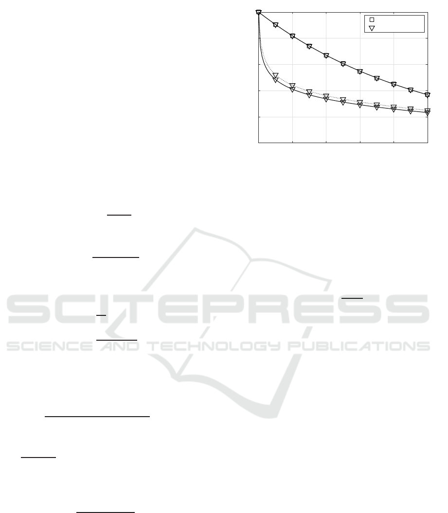
Fig. 7 shows the gap distribution functions defined in
(5) and (41). Both approaches show a close similar-
ity for different parameters of the buyer concentration
(1− α) at the buyer probability of p
e
= 10
−2
as (41)
was derived from (5).
0 20 40 60 80 100
0
0.2
0.4
0.6
0.8
1
u(k) →
k →
(1 − α) = 0.0
(1 − α) = 0.2
Figure 7: Comparison of the gap-distribution functions us-
ing (5) (dotted line) and (41) (solid line) for different pa-
rameters of (1− α) at the buyer probability of p
e
= 10
−2
.
The buyer concentration can be estimated when
analysing the probability that immediately after a
buyer in the distance k = 0 another buyer appears. In
this case the free time interval between buyers to the
cash register is zero. Taking (41) into account, the
buyer gap-density function v(k) = u(k)− u(k+ 1) re-
sults in
v(k) = u(k)

1−
k+ α
k+ 1
e
−β

. (42)
Analysing the free-time intervals with k = 0 the ex-
pression simplifies to
v(k) = u(0)· (1− α · e
−β
) . (43)
With u(0) = 1 and
e
−β
= 1− β ≈ 1 . (44)
for small values of β the probability v(0) = P(Y = 0)
equals the buyer concentration
v(0) = 1 − α . (45)
The probability v(0) is zero for non-bursty free time
intervals between buyers to the cash register and in-
creased to 50 % for bursty ones.
5 GROCERY SHOPS IN
LITHUANIA
In order to get practically relevant data regarding the
distribution of gaps, the free time intervals between
buyers to the cash register in two different shops (gro-
cery shop and supermarket) in Lithuania are studied.
The buyer probability as well as buyer concentration
derived from the obtained data allows identifying bot-
tlenecks during the payment process at the cash reg-
ister in shop sales.
Analysis of Free Time Intervals between Buyers at Cash Register using Generating Functions
47

The collected cash register data, obtained from a
single cash register of each shop, contain the opera-
tion time, the amount of goods purchased, their codes
and the prices paid by each buyer. The data collection
was carried out in June 2018 and September 2018.
Unfortunately, the cash registers do not record the
start time of the operation. Therefore, the service du-
ration time was not available from the database. To
cope with this problem the observed buyers’ service
durationswith differentquantities of goodswere anal-
ysed as shown in (Ahrens et al., 2019a). By analysing
the quantity of bought goods n
g
and the service dura-
tion t
s
the regression equation
t
s
= 1,9n
g
+ 22,8 (46)
was obtained. The equation yields that for one good
about 1,9 seconds and additionally about 22,8 sec-
onds for each buyer are required. The data were col-
lected in the grocery shop, and it is assumed that all
grocery shops as well as supermarkets have similar
performance as they are working with similar equip-
ment of cash registers and salespeople who are work-
ing at a similar intensity. Knowing the quantity of
goods and (46), the start and end times of each buyer
can be calculated. This allowed us to analyse the free
time intervals between two buyers’ service.
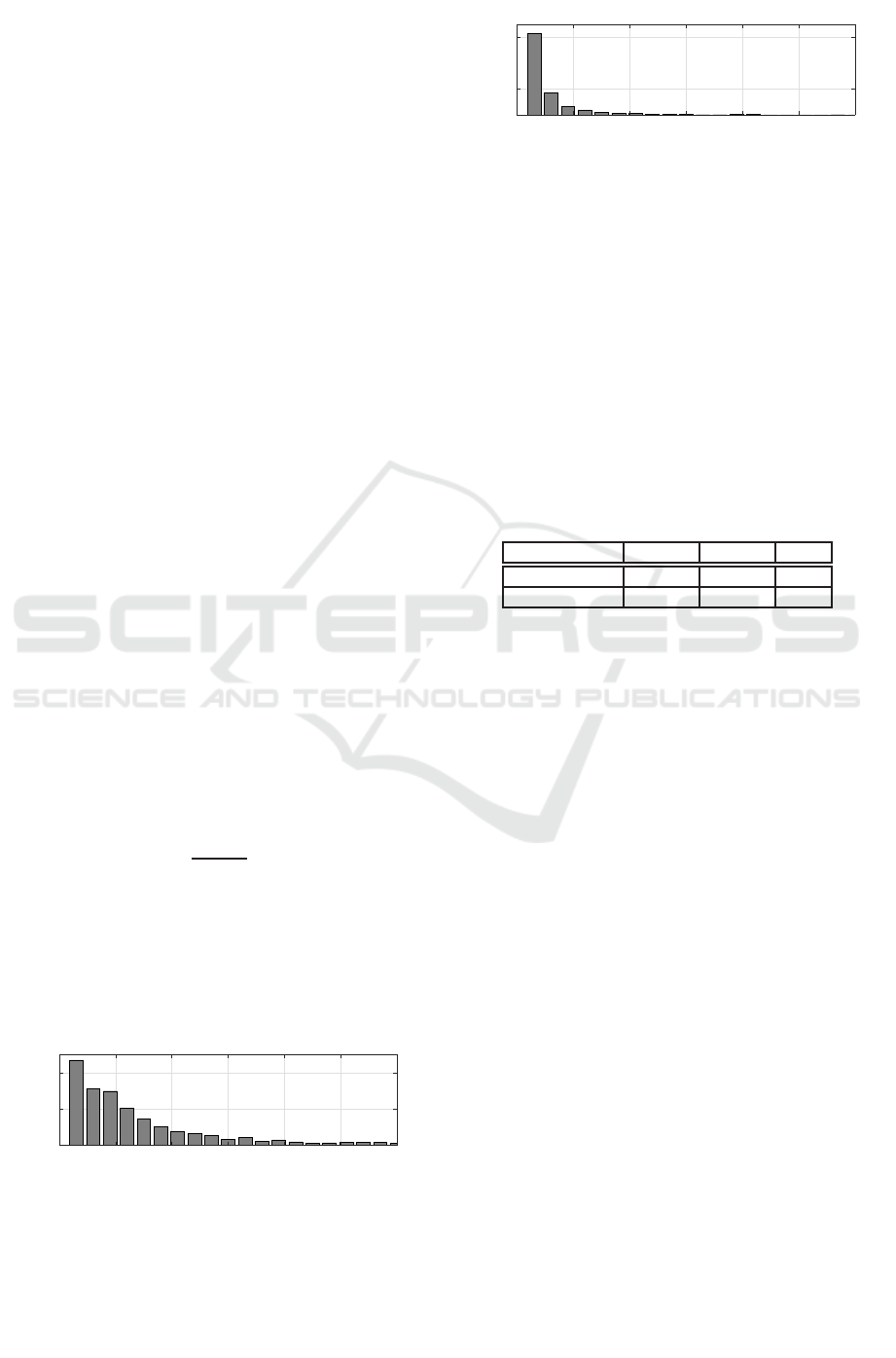
The histograms of the free time intervals at the
cash register for the grocery shop as well as the su-
permarket are given in Fig. 8 and Fig. 9. Comparing
both figures it turns out that the free times of the cash
register are more bursty in the supermarket. Here, ei-
ther short free time intervals or significantly longer
free time intervals are observed.
According to (Goh and Barab´asi, 2008), the level
of burstiness of free time intervals can be calculated
analytically and is defined as
B =
σ− m
1
σ+ m
1
, (47)
by taking the mean value m
1
(average gap length or
average length of free time intervals between two buy-
ers at the cash register) as well as the standard devi-
ation σ of the length of the free time intervals into
account. The burstiness parameter B ranges between
−1 ≤ B ≤ 1. Here, larger values of B indicate a
0 100 200 300 400 500 600
0
0.1
0.2
Probability →
t(ins) →
Figure 8: Distribution of free times of cash register
(grouped) at grocery shop.
0 100 200 300 400 500 600
0
0.2
0.6
Probability →
t(ins) →
Figure 9: Distribution of free times of cash register
(grouped) at the supermarket.
higher level of burstiness. As shown in (Ahrens et al.,
2019a), the parameter B equals the buyers’ concentra-
tion (1− α) in the range of 0 < B ≤ 1.
Tab. 1 shows the calculated level of burstiness, de-
fined by the parameter B, of free time intervals be-
tween buyers at the cash register for the two investi-
gated shops. The obtained data confirm a higher level
of burstiness in the supermarket compared with the
grocery shop when analysing the free time intervals
between buyers as shown in Fig. 8 and Fig. 9.
Table 1: Burstiness of free time intervals between buyers at
the cash register.
Shop m
1
σ B
Grocery Shop 234,1 s 620,1 s 0,45
Supermarket 96, 9 s 408,7 s 0,62
As the parameter B equals the buyers’ concentra-
tion (1−α), appropriate parameters of the underlying
gap process for modelling the free time intervals to
the cash register could be found. The results show a
slightly higher intensity, expressed by lower value m
1
and a higher buyer concentration, at the supermarket
compared with the grocery shop.
6 CONCLUSION
In this work the concept of generating functions was
applied to the field of business processes. By the theo-
retical investigations of the inter-connections between
buyers and corresponding gap-processes, a new ap-
proach based on generating functions was introduced.
Generating functions were used for the analysis of
the free time intervals between buyers to the cash reg-
ister as a part of the payment process. The proposed
parameters, namely buyer probability and buyer con-
centration, allow identifying a burstiness level. In
turn, a burstiness level serves as an indicator of bot-
tlenecks. A high level of burstiness, expressed by the
buyer concentration, increases the possibilities of bot-
tleneck emergence.
For practical verification the payment process was
analysed in two shops of different sizes in Lithuania.
PECCS 2020 - 10th International Conference on Pervasive and Parallel Computing, Communication and Sensors
48

The obtained results show that in both shops free time
intervals at the cash register are quite bursty.
Practical implementation allows concluding that
the proposed solutions are applicable to the field of
business processes.
However the research has some limitations. In this
work only two grocery shops in Lithuania were in-
vestigated. Another limitation is that only one cash
register per shop was analysed.
Further work will concentrate on the joint mod-
elling of free time intervals between buyers as well as
the payment processing time at the cash register. For
this, it is important for service quality improvement
to analyse if the found burstiness of free time inter-
vals between buyers affects the buyers’ service time.
Future research will also focus on extending the
dataset for a practical study. It includes the compar-
ison of the implemented experimental analysis with
other existing approaches. Examination of the use of
the proposed approach for large shops with numer-
ous counters will be planned and executed in order
to demonstrate the use of the approach in real-life
projects.
REFERENCES
Ahrens, A. (2000). A new digital channel model suitable
for the simulation and evaluation of channel error ef-
fects. In Colloquium on Speech Coding Algorithms
for Radio Channels, London (UK).
Ahrens, A., Purvinis, O., Hartleb, D., Zaˇsˇcerinska, J., and
Miceviˇciene, D. (2019a). Analysis of a Business En-
vironment using Burstiness Parameter: The Case of a
Grocery Shop. In International Conference on Perva-
sive and Embedded Computing and Communication
Systems (PECCS), Vienna (Austria).
Ahrens, A., Purvinis, O., and Zaˇsˇcerinska, J. (2019b).
Gap Distributions for Analysing Buyer Behaviour in
Agent-Based Simulation. In International Conference
on Sensor Networks (Sensornets), Prague (Czech Re-
public).
Chattamvelli, R. and Shanmugam, R. (2019). Generating
Functions in Engineering and the Applied Sciences.
Morgan & Claypool.
Feldmann, A. (2000). Characteristics of TCP Connection
Arrivals. In Park, K. and Willinger, W., editors, Self-
similar Network Traffic and Performance Evaluation,
chapter 15, pages 367–399. Wiley.
Goh, K.-I. and Barab´asi, A.-L. (2008). Burstiness and
Memory in Complex Systems. Exploring the Fron-
tiers of Physics (EPL), 81(4):48002.
Kessler, T., Ahrens, A., C., L., and Melzer, H.-D. (2003).
Modelling of connection arrivals in Ethernet-based
data networks. In 4rd International Conference on
Information, Communications and Signal Processing
and 4th IEEE Pacific-Rim Conference on Multimedia
(ICICS-PCM), page 3B6.6, Singapore (Republic of
Singapore).
Kresch, E. and Kulkarni, S. (2011). A poisson based bursty
model of internet traffic. In 2011 IEEE 11th Inter-
national Conference on Computer and Information
Technology, pages 255–260.
Kumar, A., Bezawada, R., Rishika, R., Janakiraman, R., and
Kannan, P. (2016). From Social to Sale: The Effects of
Firm-Generated Content in Social Media on Customer
Behavior . Journal of Marketing, 80(1):7–25.
Li, S. (1992). Generating Function Approach for discrete
Queueing Analysis with decomposable Arrival and
service Markov Chains. In IEEE International Con-
ference on Computer Communications (INFOCOM).,
pages 2168–2177, Florence (Italy).
Miceviciene, D., Purvinis, O., Glinskiene, R., and Tautkus,
A. (2018). Alternative Solution for Client Service
Management. Applied Research in Studies and Prac-
tice, 14(1):47–51.
Mittal, V. and Kamakura, W. (2001). Satisfaction, Repur-
chase Intent, and Repurchase Behavior: Investigat-
ing the Moderating Effect of Customer Characteris-
tics. Journal of Marketing Research, 38(1):131–142.
Weisstein, E. W. (1999). The CRC Concise Encyclopedia of
Mathematics. CRC Press, Boca Raton and London.
Wilhelm, H. (1976). Daten¨ubertragung (in German).
Milit¨arverlag, Berlin.
Wilhelm, H. (2018). Calculation of Error Structures in
Binary Channels with Memory. Books on Demand,
Norderstedt.
Zhang, J., Shen, F., and Waguespack, Y. (2016). Incor-
porating Generating Functions to Computational Sci-
ence Education. In International Conference on Com-
putational Science and Computational Intelligence
(CSCI)., pages 315–320, Las Vegas (USA).
Zukerman, M., Neame, T. D., and Addie, R. G. (2003).
Internet traffic modeling and future technology im-
plications. In IEEE INFOCOM 2003. Twenty-
second Annual Joint Conference of the IEEE Com-
puter and Communications Societies (IEEE Cat.
No.03CH37428), volume 1, pages 587–596.
Analysis of Free Time Intervals between Buyers at Cash Register using Generating Functions
49