Geographic Feature Engineering with Points-of-Interest from

OpenStreetMap

Adelson de Araujo, Jo

ao Marcos do Valle and N

elio Cacho

Digital Metropolis Institute, Federal University of Rio Grande do Norte, Natal, Brazil

Keywords:

Points-of-Interest, Geographic Features, OpenStreetMap, Feature Engineering.

Abstract:

Although geographic patterns have been considered in statistical modelling for many years, new volunteered

geographical information is opening opportunities for estimating variables of the city using the urban char-

acteristics of places. Studies have shown the effectiveness of using Points-of-Interest (PoI) data in various

predictive applications domains involving geographic data science, e.g. crime hot spots, air quality and land

usage analysis. However, it is hard to ﬁnd the data sources mentioned in these studies and which are the

best practices of extracting useful covariates from them. In this study, we propose the Geohunter, a repro-

ducible geographic feature engineering procedure that relies on OpenStreetMap, with a software interface to

commonly used tools for geographic data analysis. We also analysed two feature engineering procedures,

the quadrat method and KDE in which we conduct a qualitative and quantitative evaluation to suggest which

better translate geographic patterns of the city. Further, we provide some illustrative examples of Geohunter

applications.

1 INTRODUCTION

There is a growing demand for measurement and

monitoring of landscape-level patterns and processes

(Gustafson, 1998), and modern sources of data are

becoming useful for predictive analysis. Although

geographic patterns have been considered in statisti-

cal modelling for many years, new volunteered geo-

graphical information is opening opportunities for es-

timating variables of the city using the urban charac-

teristics of places. For example, when it is asked for

some inference on crime concentration within the ur-

ban space, it may be reasonable to argue that street

network may be an important predictor (Davies and

Johnson, 2015), as well as estimating air quality lev-

els where the presence of natural spaces within the

city may be useful. In this paper we detail a method-

ology to extract such covariates by using an Open-

StreetMap interface and compare two methods to de-

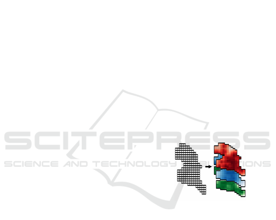
compose city data into layers of information. Our

goal is to represent the city into densities of points-

of-interest, as Figure 1 depicts.

Supported by volunteered geographical infor-

mation and data from points-of-interest (PoI), re-

searchers in many ﬁelds continue to investigate the as-

sociation between geographical patterns and the stud-

ied domain. For example, spatiotemporal crime pre-

Figure 1: Geographic features as city layers.

diction (Lin et al., 2018), energy retail (Hopf, 2018),

land usage (Estima and Painho, 2013) and several oth-

ers. With a variety of methods for representing such

patterns, researchers extract the density of PoI within

city-regions. For example, Yin et al. (Yuan et al.,

2012) classiﬁed functional regions in Beijing using

a topic modelling based technique that helps to de-

ﬁne a place as it was a document. Yuan et al. (Yin

et al., 2011) have addressed, including mobility data

on a similar topic modelling approach. Lin et al. (Lin

et al., 2018) extracted geographic features by count-

ing the number of PoI within grid cells.

Even that previous studies have examined the us-

age of geographic features, the validation of a more

appropriate feature engineering method is rarely dis-

cussed. For spatial predictions and urban analytics,

we believe that PoI density, instead of quantity, may

116

de Araujo, A., Marcos do Valle, J. and Cacho, N.

Geographic Feature Engineering with Points-of-Interest from OpenStreetMap.

DOI: 10.5220/0010155101160123

In Proceedings of the 12th International Joint Conference on Knowledge Discovery, Knowledge Engineering and Knowledge Management (IC3K 2020) - Volume 1: KDIR, pages 116-123

ISBN: 978-989-758-474-9

beneﬁt predictive modelling in many applications,

due to a few reasons. Tobler’s First Law of Geog-

raphy (TFL), also mentioned by geographers as “spa-

tial dependency”, suggests that characteristics of near

places are contiguously correlated together. Also, it is

reasonable to think that predictive models can beneﬁt

more from a diverse and balanced variable distribu-

tion, and by counting items within cells, having fell

samples may be a threaten for this, as we show.

To calculate PoI density, we evaluate the count-

based baseline method, which we refer here to as

the quadrat method, against kernel density estimation

(KDE) that generally produces relatively smoother

distributions. We evaluate these two by measuring

the spatial autocorrelation of the features provided

with Moran’s I, and spatial heterogeneity with the q-

index, which shall indicate how uneven features are

distributed. To visually compare these methods, we

conduct a qualitative assessment based on visual in-

spection of the spatial distribution for different sam-

ple sizes.

Also, from the best of our knowledge, we did

not ﬁnd that related studies show a clear and repro-

ducible geographic feature engineering procedures,

either a piece of software that would support such

analysis. For this reason, we propose and demon-

strate Geohunter, a reproducible geographic feature

engineering framework that fetches OpenStreetMap

data and calculates the density of points-of-interest

throughout the city. We implemented it as open-

source python-package, currently with the functional-

ities of (i) loading data from the OpenStreetMap API,

(ii) parse OpenStreetMap data into commonly-used

geometric-based data structures (Geopandas (Jordahl,

2014)) and (iii) to extract geographic features from

points-of-interest with the methods used in this work.

This paper is divided as follows. In Section II, we

describe some aspects of the data source, the two geo-

graphic feature engineering methods used, our evalu-

ation approach, the evaluation approach, and provide

some details about the Geohunter. In Section III, we

show the results of our experiments, both in qualita-

tive and quantitative assessments. Finally, in Section

IV, we discuss some possible outcome analysis that

illustrates the usefulness of such geographic features.

2 DATA AND METHODS

2.1 OpenStreetMap Data

Over the last decade, WEB-based GIS technolo-

gies were created to provide reliable representations

of the urban environment. Among them, Open-

StreetMap certainly gained notoriety due to its sub-

stantial community-based contributions and because

of its open data policy. It drove the growth of the Vol-

unteered Geographic Information (VGI) culture, and

many studies, e.g. (Kounadi, 2009; Camboim et al.,

2015), have assessed the quality of information on

the platform. Nowadays, one can quickly request its

data through, for example, the Overpass

API. Open-

StreetMap has a particular data model to represent ob-

jects or Points-of-Interest (PoI) composed of “nodes”,

“ways” and “relations”, and each object can be cre-

ated, tagged and veriﬁed by the community. There are

a set of deﬁned and most used tags to classify PoIs,

also referred to as “map features” (a complete de-

scription of them is provided in OpenStreetMap doc-

umentation

The Overpass API receives requests in a speciﬁc

query language (Overpass QL) and returns data con-

taining geographical coordinates and several other at-

tributes of the requested PoIs. For more details about

the structuring of these queries, we recommend the

API documentation. As mentioned, the returned ele-

ments follow the typology of (i) nodes, which deﬁnes

points in space, (ii) ways, which deﬁnes linear charac-

teristics and area boundaries, and (iii) relations, which

are used to explain how other elements work together.

An arbitrary PoI can be composed by a relation of

several ways and nodes. This typology is not directly

related to the geometric concepts of points, lines and

polygons.

The physical aspects of elements are described

by tags attached to them. Each tag is used to de-

scribe different aspects of an element, which can have

an unlimited number of tags describing them (as-

signed by the community). Furthermore, tags are

deﬁned by a pair key:value, for instance, a church

can be represented by the tag building:church, and

also by amenity:place of worship. For this paper,

we select tags with the purpose of illustrating the

method discussed further in this paper which can in-

volve a variety of PoI. Table 1 details the keys, values

and amounts of data within the boundaries of Natal,

Brazil.

2.2 Geographic Feature Engineering

Methods

For each geographic object listed in Table 1, we ex-

tract a separate feature layer which describes density

values for places in the city. These places can be de-

ﬁned following an administrative division of the city

https://wiki.openstreetmap.org/wiki/Overpass API

https://wiki.openstreetmap.org/wiki/Map Features

Geographic Feature Engineering with Points-of-Interest from OpenStreetMap

117

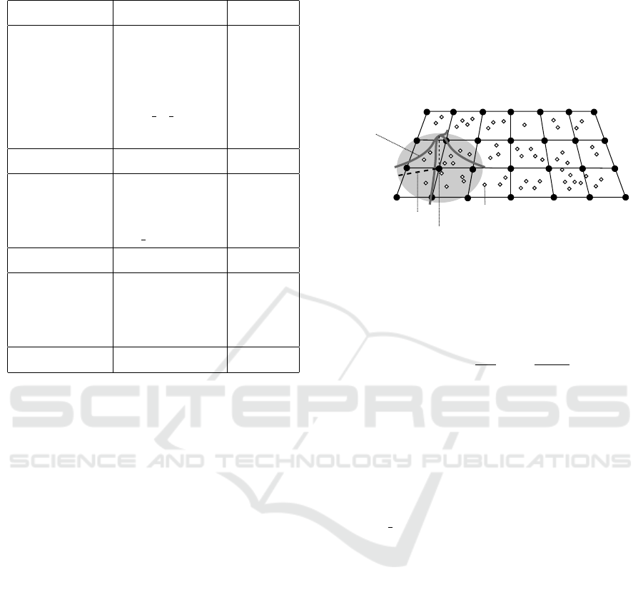
Table 1: Points-of-interest samples from data in Natal,

Brazil.

Map Features Tags Quantity

Amenity

restaurant 246

school 188

hospital 48

place of worship 154

police 39

Leisure

* 1248

Highway

primary 661

residential 8122

bus stop 417

Tourism

* 190

Natural

sand 54

wood 49

beach 16

Shop

* 1023

or an artiﬁcial grid conﬁguration. The latter has the

advantage of resolution parametrization, i.e. one can

use a ﬁner or coarser grid depending on the applica-

tion purposes. Regular geometries, such as points,

rectangles and even hexagons, are often used as the

spatial unit of analysis, or grid cell. In this paper, we

use an artiﬁcial grid composed of squares of 1km by

1km to assess the aggregation methods described be-

low. The aggregation of points within grid cells is a

relevant aspect for crafting better features.

2.2.1 Quadrat Method

A naive approach is to count the amount of PoI items

in regions of the city, which in this work, we refer to

as the quadrat method since the areas are square cells.

This method can be further generalized considering

other arbitrary geometries, using the same counting

method stated before. In the case of administrative

regions, one should normalize these values consider-

ing the respective areal density.

2.2.2 Kernel Density Estimation

The second approach consists of sampling the under-

lying probability density function, given a set of sam-

ples using a kernel. KDE is a mechanism to do so in a

non-parametric manner, ﬁrstly introduced by Rosen-

blatt (Rosenblatt, 1956) and Parzen (Parzen, 1962).

Illustrated by Figure 2, it consists of applying a kernel

function to return a density estimation of a set of arbi-

trary points, in particular for our study a grid of points

regularly spaced. Equation 1 deﬁnes it for bidimen-

sional estimation, where h is the bandwidth parameter

of the kernel function K applied, and d

x,y

(i) is the dis-

tance between all the occurrences i and the grid point

described by the coordinates x, y.

Kernelfunction

(Gaussian)

Bandwidth

Gridcell

Event

Figure 2: An illustration of Kernel Density Estimation and

its parameters. Each black point (grid cell) represents an

arbitrary place in which a kernel function applies a density

estimation around a bandwidth. For a set of events/points,

this procedure returns an array of KDE values indexed by

the identiﬁer of the cell.

f (x, y | h) =

∑

i=1

x,y

(i)

) (1)

In this sense, KDE practitioners have discussed

rules and formulas to select internal parameters. In

general, smaller bandwidths retrieve spiky distribu-

tions which may cause overﬁtting, and larger band-

widths generate too smooth surfaces, with low varia-

tion between places thus resulting in underﬁtting. Sil-

verman (Silverman, 1986) suggests a rule of thumb

of selecting bandwidth of Gaussian kernels with h =

1.06

σn

−

, considering

σ, as

σ the standard deviation

and n the sample size. Still, for other kernels, the like-

lihood maximization proposed by Jaki et al. (Jaki and

West, 2008) can be applicable. They suggest explor-

ing a parametrized version of KDE, which they called

Maximum Kernel Likelihood Estimation (MKLE),

providing an approach to select the best parameter

conﬁguration by maximizing the log-likelihood, even

providing a formula for Gaussian kernels. In a simi-

lar approach, Mohler et al. (Mohler et al., 2011) and

Hu et al. (Hu et al., 2018) suggested to search for op-

timal parameters through likelihood cross-validation.

For this study, we chose to work with the Silverman’s

method for KDE parameter selection, using the Gaus-

sian kernel. The KDE implementation we used is

from the heavily used scipy python-package(Virtanen

et al., 2020).

As mentioned, in this paper, we are working with

square grids, instead of a point-based grid. Although

some related work has applied KDE with square grids

KDIR 2020 - 12th International Conference on Knowledge Discovery and Information Retrieval

118

(using the centroid of the square to apply KDE), we

argue that the bandwidth assumes a circular format,

not square. Instead, ﬁrst, we apply KDE with a point-

based grid spaced by half of the square grid resolution

parameter. To get the resulting density estimation on

the square grid cells, we average the KDE results of

the grid points within the square grid cells.

2.3 Evaluation Method

We conduct the feature engineering approaches with

a grid resolution of 1km by 1km to quantify the in-

ﬂuence of grid cell size on the quality of feature dis-

tribution. For a quantitative evaluation, we measure

the Moran’s I for global Spatial Autocorrelation (SA)

(Anselin, 1995). We consider spatial autocorrela-

tion an important measure following the Tobler’s First

Law of Geography that suggests near places are more

similar among each other, and our purpose is to repre-

sent PoI underlying density better. On the other hand,

we measure the q-statistic for Spatial Stratiﬁed Het-

erogeneity (SSH) to handle the traditional concept in

the geography of spatial heterogeneity, in which Leit-

ner et al. (Leitner et al., 2018) suggests that local

uniqueness should condition generalizations and pat-

tern extraction. Also, we conduct a qualitative analy-

sis by visual inspection of the feature distribution gen-

erated by the baseline and by KDE, with two feature

items taken from different sample sizes.

The Moran’s I is expressed in equation 2, where

N is the number of spatial units index by i and j, x the

variable of interest, ¯x its mean, w

i j

a matrix of spatial

weights, and W the sum of all weights in w

i j

. It quan-

tiﬁes how much neighbours cells does correlate with

each other, and it ranges from -1 to 1. The metric

interpretation indicates that one means perfect clus-

tering (high spatial autocorrelation) of similar values,

-1 means perfect dispersion, and 0 means perfect ran-

domness (no spatial autocorrelation) (Anselin, 1995).

I =

∑

i j

− ¯x)(x

− ¯x)

∑

− ¯x)

(2)

The q-statistic is expressed in Equation 3, where

L is the number of strata, N the size of the population

and σ

the variance of the attribute. It assesses data

heterogeneity among grid stratiﬁcation, and it varies

from 0 to 1. The strata are sets of grid cells, for

instance, cells within the administrative neighbour-

hoods. A value close to 0 indicates that variances

within strata are similar (homogeneous). Conversely,

when values are close to 1 stratus’s variation are more

heterogeneous among each other, thus more prone to

represent different patterns among places. For further

details on the importance of measuring the q-statistic,

we refer to (Wang et al., 2016) that provide seminal

arguments and additional formal description on it.

q = 1 −

Nσ

∑

h=1

(3)

2.4 The GEOHUNTER Python-package

To provide an open-source tool for other researchers

to extract geographic features and to ensure experi-

ment reproducibility, we developed the Geohunter

python-package. It aims to obtain and parse data

from OpenStreetMap to robust geospatial data struc-

tures, as provided by the GeoPandas package(Jordahl,

2014).

The workﬂow of Geohunter starts with a bound-

ing area, which can be taken from an input ﬁle for

the city shape (spatially encoded ﬁles, such as shape-

ﬁle or GeoJSON) or we can get it from the Geo-

hunter, setting a bounding box and request it with

its OpenStreetMap unique tags. One can easily re-

quest any data, including PoI and city shapes, by call-

ing our API facade, setting the tags and the values

wanted. Then, Geohunter parse and execute the Over-

pass query, get the results and parse as GeoPandas’

GeoDataFrame.

The grid object also uses the city shape, and Geo-

hunter provides functions for generating square grid

bounded by a particular area. Then, the grid and PoI

are used as input for the feature engineering method,

considering quadrat and KDE methods. By default,

we use Silverman’s method to retrieve KDE parame-

ters used, as mentioned before. The output is a matrix,

where each column represents a geographic feature,

and each row indicate a tuple of feature values for a

given grid cell. In the package’s GitHub repository,

there are a few examples on how to use Geohunter,

including to reproduce or clarify the experiment de-

scribed in this paper.

3 RESULTS

Using the dataset gathered from Natal, Brazil, we

extracted geographic features using both methods,

quadrat and KDE. Since there is a diverse set of sam-

ple sets, ranging from beaches with 16 samples, to

residential streets with 8122, we argue that useful

comparisons can be made on different scenarios.

https://geohunter.readthedocs.io/en/latest/

Geographic Feature Engineering with Points-of-Interest from OpenStreetMap

119

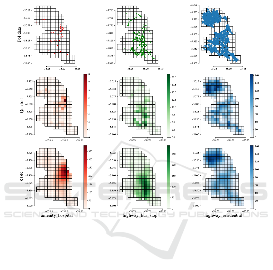
Figure 3: The density of PoI data (ﬁrst row) using the quadrat method (second row) and KDE (third row) for three categories.

Hospitals map with 48 points in red is representative because it shows that with a few samples, the method visually differs

signiﬁcantly. Bus stops map with 417 items in green also follows such difference. On the right side, residential streets map

with 8122 samples in blue shows that with a massive amount of points, it is hard to detect a difference in feature distribution

visually, but KDE still generated a smoother map.

3.1 Qualitative Assessment

To demonstrate the visual effect of the extracted fea-

tures in a grid with 1km by 1km cells, we present

the Figure 3. It has the spatial density of three PoI

items (48 hospitals in red, 417 bus stops in green

and 8122 residential streets in blue), as well as their

feature distribution with the quadrat method (middle

row) and KDE (last row). We pick these three because

they represent different sample sizes and support fur-

ther inspections on possible sample size-dependent

behaviour. Note that with fewer samples, the quadrat

method is more likely to have neighbour cells with to-

tally different values when comparing to KDE. How-

ever, when having a massive amount of samples, the

maps become more similar to each other. With this vi-

sual inspection, one can ﬁnd that KDE-based features

are relatively more parsimonious than quadrat ones, in

all three cases, even when more data is available. In a

possible question involving what is the coverage area

of hospitals, we argue that the KDE ones are more

likely to represent the reality.

3.2 Quantitative Assessment

In section 2.3, we discussed that the quantitative eval-

uation conducted in this article is guided by two es-

sential concepts of geography, spatial autocorrelation

through Moran’s I, and spatial heterogeneity, calcu-

lated through q-statistic (Wang et al., 2016). These

metrics are relevant to evaluate our hypothesis that

KDE is, in fact, more meaningful for PoI density rep-

resentation, following the geography rules described

earlier.

KDIR 2020 - 12th International Conference on Knowledge Discovery and Information Retrieval

120

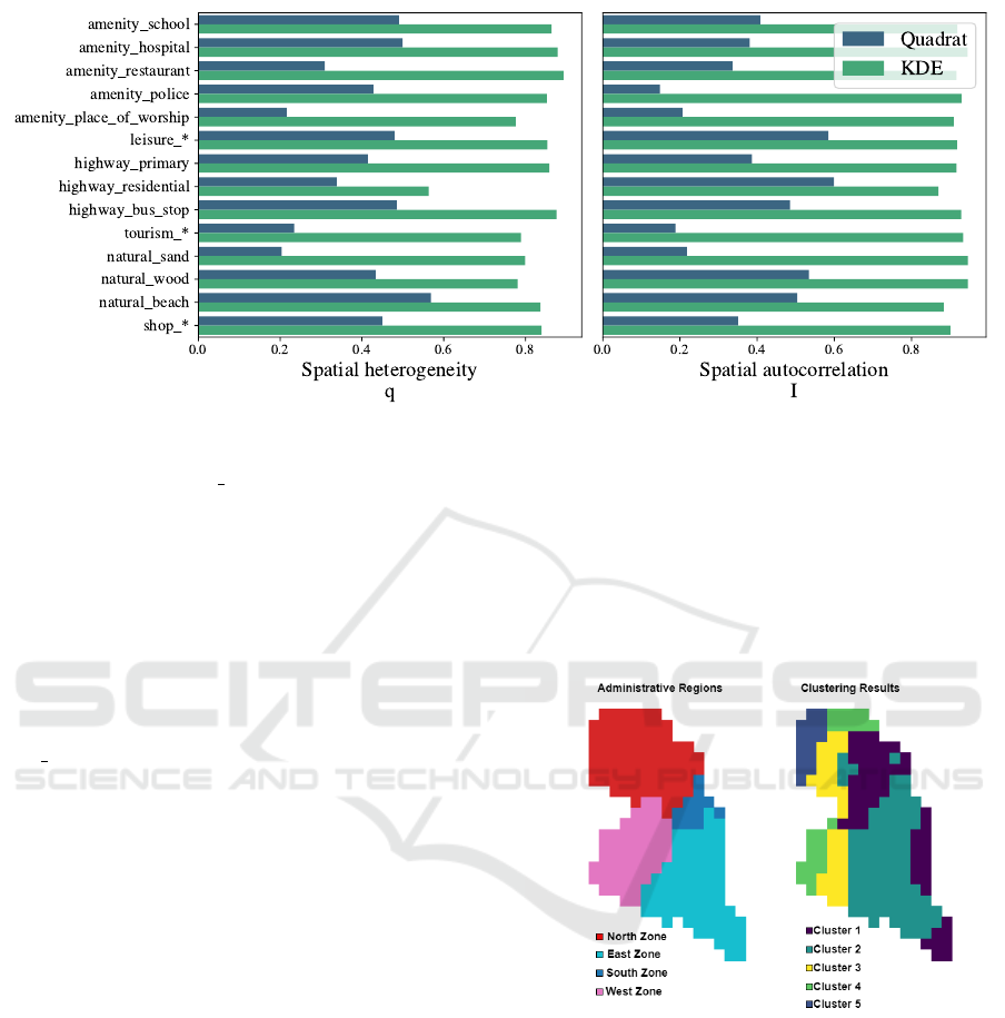
Figure 4: Comparison between the quadrat method and KDE regarding spatial heterogeneity (q) and spatial autocorrelation

(I) for all features extracted. Clearly, KDE performed better than quadrat in both metrics, even in cases where more samples

are available (e.g. highway residential).

In this sense, we report in Figure 4 the results of

these metrics for the quadrat and KDE methods, with

the grid resolution of 1km by 1km. Note that KDE

overcomes quadrat-based features in all scenarios,

with high values of both q and I, which indicate that

features extracted with KDE have higher spatial au-

tocorrelation and heterogeneity between cells. Such

a pattern was noticed even when massive amounts of

samples are available, e.g. residential streets (high-

way residential).

4 DISCUSSION

In Section II, we mentioned that results obtained us-

ing the Geohunter Package can be used as input for

a diverse set of predictive algorithms. To illustrate

some of the possible applications of using these fea-

tures, here we provide some examples on spatial pat-

tern analysis of urban spaces using geographic fea-

tures.

First, we used K-means on Geohunter’s output for

the city of Natal using Table 1 features. For com-

parison reasons, K-means was performed with ﬁve

clusters, similar to the same number of administra-

tive regions in Natal, which is four. Figure 5 shows

the administrative regions (left) and the clustering re-

sults (right). It is possible to assess the difference be-

tween city characteristics in both images. Using the

clustering results, we have some areas of resemblance

in an inter-regional fashion. Bodies of water (tightly

related to touristic areas), commercial zones and sub-

urbs (represented by clusters 1, 2 and 3 respectively)

are related to various administrative regions of the

city. We also argue that this output is more useful than

traditional counting data obtained by cities census, at

least for this type of application. Other example is

illustrated in Figure 6, where we show three cluster

of the city given the three features early mentioned,

hospitals, bus stops and residential streets.

Figure 5: Comparison between Natal’s administrative areas

(left) and the result of clustering using geographic features

acquired from Geohunter (right).

Also, as stated before, with Geohunter, it is possi-

ble to obtain the density of several features in the city.

This can be used, for example, to analyse the density

of police stations or hospitals in it, which is useful in-

formation to city planners to do decisions based on.

Also, it is possible to make other analysis, such as,

the relation between city facilities (hospitals, schools,

police stations) and crime spots, air pollution density,

trafﬁc, agglomerations and several other urban phe-

nomena.

Geographic Feature Engineering with Points-of-Interest from OpenStreetMap

121

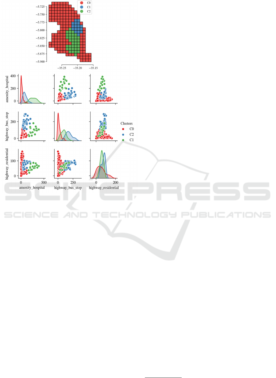
Figure 6: Clustering three zones of the city considering hos-

pitals, bus stops and residential streets. Above, note the spa-

tial distribution of the clusters, and below, the distribution

of the features for each cluster. The area C0 is characterized

as with almost no hospitals, a few bus stops and a varying

amount of residential streets, while C1 and C2 are easily

distinguished by the number of bus stops and hospitals.

5 CONCLUSION

In this paper, we proposed a reproducible framework

for geographic feature engineering in which future

work can rely on to analyse geographic patterns of ur-

ban spaces with an easy interface to OpenStreetMap.

We assessed two spatial aggregation methods regard-

ing their spatial heterogeneity and autocorrelation. In

our experiments, we provided evidence that the usage

of the KDE, if compared with the quadrat method,

has much to contribute in terms of urban represen-

tation and feature engineering. Also, we presented

the Geohunter python-package to create an interface

with OpenStreetMap data and a heavily used geospa-

tial tool (GeoPandas (Jordahl, 2014)). We provided a

brief example using the features to illustrate its appli-

cability. For future work, we suggest taking these fea-

tures and applying for environmental and urban pre-

dictions and experimenting with different grid reso-

lution and parameter settings. Modern data sources

support uncovering more geographical patterns, and

we argue that is it time to pursue ubiquitous analysis.

ACKNOWLEDGEMENTS

This work is supported by the SmartMetropolis

and

the Laboratory for Public Budget and Policies (LOPP)

of the Public Ministry of the State of Rio Grande do

Norte (MPRN).

REFERENCES

Anselin, L. (1995). Local indicators of spatial associa-

tion—lisa. Geographical analysis, 27(2):93–115.

Camboim, S. P., Bravo, J. V. M., and Sluter, C. R. (2015).

An investigation into the completeness of, and the

updates to, openstreetmap data in a heterogeneous

area in brazil. ISPRS International Journal of Geo-

Information, 4(3):1366–1388.

Davies, T. and Johnson, S. D. (2015). Examining the rela-

tionship between road structure and burglary risk via

quantitative network analysis. Journal of Quantitative

Criminology, 31(3):481–507.

Estima, J. and Painho, M. (2013). Exploratory analysis

of openstreetmap for land use classiﬁcation. In Pro-

ceedings of the second ACM SIGSPATIAL interna-

tional workshop on crowdsourced and volunteered ge-

ographic information, pages 39–46. ACM.

Gustafson, E. J. (1998). Quantifying landscape spatial

pattern: what is the state of the art? Ecosystems,

1(2):143–156.

Hopf, K. (2018). Mining volunteered geographic informa-

tion for predictive energy data analytics. Energy In-

formatics, 1(1):4.

Hu, Y., Wang, F., Guin, C., and Zhu, H. (2018). A spatio-

temporal kernel density estimation framework for pre-

dictive crime hotspot mapping and evaluation. Ap-

plied geography, 99:89–97.

Jaki, T. and West, R. W. (2008). Maximum kernel like-

lihood estimation. Journal of Computational and

Graphical Statistics, 17(4):976–993.

Jordahl, K. (2014). Geopandas: Python tools for geographic

data. URL: https://github. com/geopandas/geopandas.

Kounadi, O. (2009). Assessing the quality of openstreetmap

data. Msc geographical information science, Univer-

sity College of London Department of Civil, Environ-

mental And Geomatic Engineering.

Leitner, M., Glasner, P., and Kounadi, O. (2018). Laws of

Geography. Oxford University Press, United King-

dom.

Lin, Y.-L., Yen, M.-F., and Yu, L.-C. (2018). Grid-based

crime prediction using geographical features. ISPRS

International Journal of Geo-Information, 7(8):298.

https://smartmetropolis.imd.ufrn.br/

KDIR 2020 - 12th International Conference on Knowledge Discovery and Information Retrieval

122

Mohler, G. O., Short, M. B., Brantingham, P. J., Schoen-

berg, F. P., and Tita, G. E. (2011). Self-exciting point

process modeling of crime. Journal of the American

Statistical Association, 106(493):100–108.

Parzen, E. (1962). On estimation of a probability density

function and mode. The annals of mathematical statis-

tics, 33(3):1065–1076.

Rosenblatt, M. (1956). Remarks on some nonparametric

estimates of a density function. The Annals of Mathe-

matical Statistics, pages 832–837.

Silverman, B. W. (1986). Density estimation for statistics

and data analysis.

Virtanen, P., Gommers, R., Oliphant, T. E., Haberland, M.,

Reddy, T., Cournapeau, D., Burovski, E., Peterson,

P., Weckesser, W., Bright, J., et al. (2020). Scipy

1.0: fundamental algorithms for scientiﬁc computing

in python. Nature methods, 17(3):261–272.

Wang, J.-F., Zhang, T.-L., and Fu, B.-J. (2016). A measure

of spatial stratiﬁed heterogeneity. Ecological Indica-

tors, 67:250–256.

Yin, Z., Cao, L., Han, J., Zhai, C., and Huang, T. (2011).

Geographical topic discovery and comparison. In

Proceedings of the 20th international conference on

World wide web, pages 247–256. ACM.

Yuan, J., Zheng, Y., and Xie, X. (2012). Discovering re-

gions of different functions in a city using human

mobility and pois. In Proceedings of the 18th ACM

SIGKDD international conference on Knowledge dis-

covery and data mining, pages 186–194. ACM.

Geographic Feature Engineering with Points-of-Interest from OpenStreetMap

123