Classifying Incomplete Vectors using Decision Trees

Bhekisipho Twala

, Raj Pillay

and Ramapulana Nkoana

Faculty of Engineering and the Built Environment, Durban University of Technology, Durban 4000, South Africa

City of Johannesburg, Group Governance Department, Johannesburg 2000, South Africa

CSIR, Climate Change Modelling Group, Pretoria 0001, South Africa

Keywords: Incomplete Data, Supervised Learning, Decision Trees, Logit Models, Classification Accuracy.

Abstract: An attempt is made to address the problem of classifying incomplete vectors using decision trees. The essence

of the approach is the proposal that in supervised learning classification of incomplete vectors can be

improved in probabilistic terms. This approach, which is based on the a priori probability of each value

determined from the instances at that node of the tree that has specified values, first exploits the total

probability and Bayes’ theorems and then the probit and logit model probabilities. The proposed approach

(developed in three versions) is evaluated using 21 machine learning datasets from its effect or tolerance of

incomplete test data. Experimental results are reported, showing the effectiveness of the proposed approach

in comparison with multiple imputation and fractioning of instances strategy.

1 INTRODUCTION

Datasets are seldom complete and this can introduce

biases, hence, incorrect predictions when using

supervised machine learning models. The three most

common tasks when dealing with incomplete data is

to investigate the proportion (how much information

is lost because of missing), the pattern (which values

are missing) and the law generating the missingness

(whether missingness is related to the study

variables). When missing values are confined to a

single variable we have a univariate pattern or

univariate nonresponse. When the same cases miss

instances on a set of variables we have a multivariate

nonresponse pattern. The monotonic pattern occurs

when missing a subject implies that other variables

will be missing as well. Arbitrary patterns occur when

any set of variables may be missing for any unit.

Another missing data pattern could occur when two

sets of variables are never jointly observed. Finally,

there are cases where no clear pattern could occur

(general non-response). (Little and Rubin, 1987;

Schafer, 1996).

Understanding the law generating the missing

values seems to be the most important task since it

facilitates how the missing values could be estimated

more efficiently. If data are missing completely at

https://orcid.org/0000-0000-3452-9581

random (MCAR) or missing at random (MAR), we

say that missingness is ignorable.

For example, suppose that you are modelling

systems engineering as a function of project

management requirements. There may be no

particular reason why some systems engineers told

you about their project management requirement and

others did not. Such data is considered to be MCAR.

Furthermore, the requirements of managing a project

may not be identified due to a given systems

engineering task. Such data are considered to be

MAR. MAR essentially says that the cause of missing

data (project management requirements) may be

dependent on the observed data (systems

engineering) but must be independent of the missing

value that would have been observed. It is a less

restrictive model than MCAR, which says that the

missing data cannot be dependent on either the

observed or the missing data. For data that is

informatively missing (IM), we have non-ignorable

missingness (Little and Rubin, 1987), that is, the

probability that a successful project is missing

depends on the unobserved value of an engineering

system itself. In other words, the missing data

mechanism is related to the missing values. For

example, software project managers may be less

likely to reveal projects with high defect rates.

Twala, B., Pillay, R. and Nkoana, R.

Classifying Incomplete Vectors using Decision Trees.

DOI: 10.5220/0010146304550463

In Proceedings of the 12th International Joint Conference on Computational Intelligence (IJCCI 2020), pages 455-463

ISBN: 978-989-758-475-6

455

When missing features are encountered, some ad

hoc approaches such as deleting the data vectors with

missing values or imputation have been utilized by

researchers to form a complete-data format. Deletion

does not add bias if the data are missing completely

at random (MCAR) but can lower the confidence of

your supervised machine learning models because the

sample size is reduced. Imputation means that

predicted or representative values are filled in place

of the missing data. If data are MCAR, imputation

tends to produce and overconfident model due to the

uncertainty that the values are artificially imputed.

Some researchers have used sophisticated built-in

system procedures to deal with the incomplete data

problem such as C4.5 (Quinlan, 1993) and CART

(Breiman et al., 1984) and probability estimation

(Khosravi et al., 2020).

The major contribution of the paper is the

proposal that classifying incomplete vectors with the

decision tree classifier can be performed in

probabilistic terms. This approach is based on the a

priori probability of each value determined from the

instances at that node of the tree that has specified

values.

The rest of the paper is organised as follows.

Section 2 briefly discusses the details of five missing

data techniques (MDTs) that are used in this paper.

The framework of the proposed probabilistic method

is also introduced and described. Section 3

empirically evaluates the robustness and accuracy of

the new technique in comparison with multiple

imputation and Quinlan’s fractioning of cases

strategy on twenty-one machine learning domains.

We close with a discussion and conclusions, and then

directions for future research

2 DECISION TREES AND

MISSING DATA

DTs are a simple yet successful technique for

supervised classification learning. A DT is a model of

the data that encodes the distribution of the class label

in terms of the predictor attributes; it is a directed,

acyclic graph in the form of a tree. The root of the tree

does not have any incoming edges. Every other node

has exactly one incoming edge and zero or more

outgoing edges. If a node n has no outgoing edges we

call n a leaf node, otherwise, we call n an internal

node. Each leaf node is labelled with one class label;

each internal node is labelled with one predictor

attribute called the splitting attribute. Each edge e

originating from an internal node n has a predicate q

associated with it where q involves only the splitting

attribute of n.

Several methods have been proposed in the

literature to treat missing data when using DTs.

Missing values can cause problems at two points

when using DTs; 1) when deciding on a splitting point

(when growing the tree), and 2) when deciding into

which child node each instance goes (when

classifying an unknown instance). Methods for taking

advantage of unlabelled classes can also be

developed, although we do not deal with them in this

paper, i.e., we are assuming that the class labels are

not missing.

The next section describes two MDTs that have

been proposed in the literature to treat missing data

when using DTs. These techniques are also the ones

used in the simulation study in Section 3.

2.1 Multiple Imputation

Multiple imputation is one of the most attractive

methods for general purpose handling of missing data

in multivariate analysis. (Rubin, 1987; 1996)

described MI as a three-step process. First, sets of M

plausible values (M=5 in Figure1) for missing

instances are created using an appropriate model that

reflects the uncertainty due to the missing data. Each

of these sets of plausible values is used to “fill-in” the

missing values and create M “complete” datasets

(imputation). Second, each of these M datasets can be

analyzed using complete-data methods (analysis).

Finally, the results from the M complete datasets are

combined, which also allows the uncertainty

regarding the imputation is taken into account

(pooling or combining).

There are various ways to generate imputations.

(Schafer, 1997; Schafer and Graham, 2002) has

written a set of general-purpose programs for MI of

continuous multivariate data (NORM), multivariate

categorical data (CAT), mixed categorical and

continuous (MIX), and multivariate panel or clustered

data (PNA). These programs were initially created as

functions operating within the statistical languages R.

NORM includes an Expectation-maximization

(EM) algorithm for maximum likelihood estimation of

means, variance and covariances. NORM also adds

regression-prediction variability by using a Bayesian

procedure known as data augmentation (Tanner and

Wong, 1987) to iterate between random imputations

under a specified set of parameter values and random

draws from the posterior distribution of the parameters

(given the observed and imputed data). These two

steps are iterated long enough for the results to be

reliable for multiple imputed datasets. The goal is to

NCTA 2020 - 12th International Conference on Neural Computation Theory and Applications

456

have the iterates converge to their stationary

distribution and then to simulate an approximately

independent draw of the missing values (Wu, 1983).

This is the approach we follow in the paper, which we

shall now call EM multiple imputation (EMMI). The

algorithm is based on the assumptions that the data

come from a multivariate normal distribution and are

MAR

2.2 Fractioning of Cases (FC)

Supervised learning algorithms, like fractioning of

cases (FC), have been successfully used to handling

incomplete data although they are generally more

complex than ordinary statistical techniques.

Supervised learning is a machine learning technique

for learning a function from training data. The

training data consists of pairs of input objects

(typically vectors), and desired outputs. The output of

the function can be a continuous value (called

regression) or can predict a class label of the input

object (called classification).

Quinlan, (1993) borrows the probabilistic

approach by Cestnik et al., (1987) by “fractioning”

cases or instances based on a priori probability of

each value determined from the cases at that node that

has specified values. Quinlan starts by penalising the

information gain measure by the proportion of

unknown cases and then splits these cases to both

subnodes of the tree as described briefly below.

The learning phase requires that the relative

frequencies from the training set be observed. Each

case of, say, class C with an unknown attribute value

A is substituted. The next step is to distribute the

unknown examples according to the proportion of

occurrences in the known instances, treating an

incomplete observation as if it falls all subsequent

nodes.

For classification, Quinlan’s (1993) technique is

to explore all branches below the node in question and

then take into account that some branches are more

probable than others. Quinlan further borrows

Cestnik et al. (1987) strategy of summing the weights

of the instance fragments classified in different ways

at the leaf nodes of the tree and then choosing the

class with the highest probability or the most probable

classification. When a test attribute has been selected,

the cases with known values are divided into the

branches corresponding to these values. The cases

with missing values are, in a way, passed down all

branches, but with a weight that corresponds to the

relative frequency of the value assigned to a branch.

Both strategies for handling missing attribute

values are used for the C4.5 system. Unfortunately,

for FC, there are no assumptions made about the law

generating the missing values. Thus, we shall assume

that the data is MCAR.

2.3 Probability Estimation Approach

The proposed probabilistic approach to missing

attribute values follows both branches from each node

if the value of the attribute being branched on is not

known.

Given  mutually exclusive events 



,…,



whose probabilities sum to unity, then









∑



























(2.1)

where  is an arbitrary event and 











is the

conditional probability of Y assuming



. This is the

theorem of total probability.

The total probability theorem and the definition of

conditional probability (introducing an arbitrary

event Z) may be used to derive











∑







,





















(2.2)

The missing value problem addressed in this paper

can be defined as follows:

Given: A decision tree, a complete set of training

data, and a set of instances for testing described with

attributes and their values. Some of the attribute

values in the test instances are unknown.

Find: A classification rule for a new instance using

the tree structure given that it has an unknown

attribute value and by using the known attribute

values.

Let  be the attribute associated with a particular

node of the tree that could either be discrete or

numerical. A discrete attribute has a certain number

of possible values  and a continuous attribute may

attain any value from a continuous interval. Each

node is split into two sons (left and right sons). Hence,

a new instance could either go to the left (L) or the

right (R) of each internal node. Further, let  be the

binarised value for attribute. Let C denote a class

and let there be  classes, =1,…,.

The total probability theorem is used to predict the

class membership of an unknown attribute value by

computing the conditional probability of a class 

given the evidence of known attribute values.

For individual j, divide the attributes in the tree

into classes for both 

(the known attribute values)

and 

(the missing attribute values). Then





=

∑





, (2.3)

where the sum is over all possible combinations of

values that branch to the left (L) or right (R) at each

Classifying Incomplete Vectors using Decision Trees

457

respective internal node, taken by the vector of the

missing attribute values 

. For the unknown attribute

values, the unit probability may be distributed across

the various leaves to which the new instance could

belong. These probabilities are going to be estimated

to each class in three ways as explained below.

For illustration purposes, suppose that from

Figure 1 the values for 



(categorical attribute) and





(numerical attribute) are missing, and 



is the

only numeric attribute with non-missing values.

Figure 1: Example of binary decision.

Figure 1 An example of a binary decision tree

from a set of 40 training instances that are represented

by three attributes and accompanied by two classes.

Figures in brackets are the number of instances in

each terminal node for class 1 and 2, respectively.

Figures in italic represent training data instances that

branch to the right or the left of each internal node at

each respective cut-off point. For purposes of space,

we shall only look at the second case.

First Case: Class membership for a new instance is

predicted given that it will branch to the left of the

internal node 













), given that both 



and 



have unknown attribute values.

The probability that the predicted class

membership will be class 1 given that it branches to

the left at internal attribute 2



















is computed

as:

















=













,





,

















,



























,





,

















,



























,





,

















,



























,





,

















,













(2.4)

Similarly,

















=













,





,

















,



























,





,

















,



























,





,

















,



























,





,

















,













=1−















(2.5)

Second Case: Class membership for a new instance

given that it will branch to the right of the internal

node 













is predicted, given that both 



and 



have unknown attribute values. The class with the

biggest probability is selected. We can define the

probability that the predicted class membership will

be class 1 given that it branches to the right of internal

attribute 2 2



















and follows a similar pattern

as the first case.

2.3.1 Full Estimation of Probabilities from

the Training Set (TSPE)

From Figure 1, there is 1 class and 1 individual

associated with 













<4061.5



, 













<3.5

















<21.5



, 1 class and 1 individual with 











, 





and so on. Also, one of the 7 





individuals

(i.e. 



<4061.5) has 





, 





, another 1 has 





, 





and so on. Therefore, the estimated probability of

membership of class 1 is given by:

















=



































+



































+





































+



































=0.839 (2.6)

Following from (2.6), 















=1−

















=0.161where 















and 















are both estimated from the proportion of instances in

the training set for which this is true, respectively.

2.3.2 Approximation of Probabilities

Estimated from Decision Tree (DTPE)

From figure 1, the estimated probability of

membership of class 1 is given by:

















=













,







































,

























(2.7)

where















,







=













,





























,







+













,





























,







=



+



=

(17,1)

(2,5)

(4,2)

(7,2)

>3.5

<3.5

<4061.5

>4061.5

>21.5 <21.5

NCTA 2020 - 12th International Conference on Neural Computation Theory and Applications

458

therefore,

















≈



+



=0.828

Using (2.7),

















=













,

























+













,

























=1−















=0.172

2.3.3 Full Estimation of Probabilities from

Training Data using Binary and

Multinomial Logit Models (LPE)

In this sub-section, the estimation of probabilities for

the new probabilistic method is improved by using

logistic regression (Agresti 1990; McCullough and

Nelder, 1990) and multinomial logit techniques

(Hosmer and Lemeshow, 1989; Long, 1998),

individually. The binary logit model is used to

estimate probabilities for those datasets that have two

classes with the latter used to estimate probabilities

for datasets with more than two classes.

McCullugh and Nelder (1990) discuss how

classification and discrimination problems as forms

of modelling the relationship between a categorical

variable and various explanatory variables are

considered. It was shown how logistic regression

techniques could be used for such a task. For

example, suppose that there are two classes, 1 and 2,







,





and v attribute variables 



,…,



. Then the

probability that an object with values 



,…,



belongs to class 1 as a logistic function of 



,…,



could be modelled:



























⋯





















⋯







(2.8)

and then estimate the unknown parameters 



from

the training data on objects with known

classifications.

Binary logit models describe the relationship

between a dichotomous response variable and a set of

explanatory variables of any type. The explanatory

variables may be continuous or categorical. Binary

logit tries to model the logarithmic odds-ratio for the

classification (dependent variable C) as a linear

function of the  ‘input’ or attribute variables





=



,



,…,



For purposes of this paper, the binary logit model

was not used to estimate probabilities based on all the

attributes given in the dataset, but to estimate only the

unknown probabilities of the given attributes

specifically related to the problem. For each specific

attribute, the values of the instances were made binary

in accordance to the branching of that particular value

at the internal node of the tree, i.e., whether the value

branched to the left or the right at the internal node.

For example, if the value branched to the left of the

internal node of interest, it was recorded as 1.

Otherwise, it was recorded as 2.

For the two-class example discussed in Section

2.3.1, the conditional probabilities involving only the

class given in equations 3.3 and 3.4, could be

estimated by the binary logit model in terms of the log

odds ratio in the form:

log

































=



+









(2.9)

where 



is the k dimensional coefficient vector. The

odds ratio is a factor of how many times the event (



)

is more likely to happen than the event (



) given the

knowledge of A.

For an example 













,





,







is estimated by

log

















,





,























,





,







=



+









+









+









Although the binary logit model finds the best

‘fitting’ equation just as the linear regression does, the

principles on which it does so are different. Instead of

using the least-squares deviations criterion for the

best fit, it uses a maximum likelihood method, which

maximises the probability of getting the observed

results given the fitted regression coefficients.

We have talked about a model that could be used

for a dependent variable that has only two possible

categories or two classes for the example. We shall

now look at a model that will be able to handle a

three-classes or more type of problem. These models

are known as multinomial logit regression (MLR) and

have the following form:





=



















∑























for =1,…,+1 (2.10)

which will automatically yield probabilities that add

up to one for each j.

To identify the parameters of the model, 



set to 0 (a zero vector) as a normalisation procedure

and thus:





























∑























(2.11)

In the multinomial logit model, the assumption is that

the log-odds of each response follow a linear model.

Thus, the j

logit has the following form:

log





















=











(2.12)

Classifying Incomplete Vectors using Decision Trees

459

where 



is a vector of regression coefficients for

=1,…,. This model is analogous to the LR model,

except that the probability distribution of the response

is multinomial instead of binomial and there are k

equations instead of one. The k multinomial logit

equations contrast each of categories =1,…, with

category k+1, whereas a single logistic regression

equation is a contrast between successes and failures.

If k = 1 the multinomial logit model reduces to the

usual binary regression model. The multinomial logit

model is, in fact, equivalent to running a series of

binary logit models (Hosmer and Lemeshow, 1989,

Long, 1998).

The crucial difference between FC and the

proposed approach is that whereas the proposed

procedure considers only those instances belonging to

that particular class for which an unknown instance

would be classified, FC considers all the instances

branching to that particular leaf node whose class is

being predicted, and which would be given at the

particular leaf node. For illustration purposes on how

the proposed technique works, the reader is referred

to Twala (2005).

3 EXPERIMENTS

3.1 Experimental Set-up

In this section, the behaviour of the three proposed

procedures against two approaches that have

previously been proposed for handling unknown

attribute values in test data when using DTs is

explored utilizing twenty-one datasets obtained from

the machine learning repository (Murphy and Aha,

1992).

The two current methods selected (EMMI and

FC) are the ones which provided very good results in

the experiments carried out in (Twala, 2005; Twala et

al., 2008). The main objective is to compare the

performance of the proposed methods(TSEPE, DTPE

and LPE) with current approaches to deal with the

problem of incomplete test data in terms of smoothed

error rate and computational cost. EMMI is used as a

baseline as it was clearly ‘the winner’ in previous

experiments (Twala and Cartwright, 2005; Twala et

al., 2005). Besides, since the proposed algorithm is

superficially similar to FC (one of the most well-

known machine learning algorithm), it was of

importance to explore how accurate it is relative to

FC.

To perform the experiment each dataset was split

randomly into 5 parts (Part I, Part II, Part III, Part IV,

Part V) of equal (or approximately equal) size. 5-fold

cross-validation was used for the experiment. For

each fold, four of the parts of the instances in each

category were placed in the training set, and the

remaining one was placed in the corresponding test.

The same splits of the data were used for all the

methods for handling incomplete test data.

To simulate missing values on attributes, the

original datasets are run using a random generator

(for MCAR) and a quintile attribute-pair approach

(for both MAR and IM, respectively). Both of these

procedures have the same percentage of missing

values as their parameters. These two approaches are

run to get datasets with four levels of the proportion

of missingness p, (0%, 15%, 30% and 50%).

For each dataset, two suites were created. First,

missing values were simulated on only one attribute.

Second, missing values were introduced uniformly on

all the attribute variables. For the second suite, the

missingness was evenly distributed across all the

attributes. This is the case for the three missing data

mechanisms, which from now on shall be called

MCARuniva, MARuniva, IMuniva (for the first

suite) and MCARunifo, MARunifo, IMunifo (These

procedures are described in Twala (2005).

3.2 Experimental Results

The performance of the MDTS is summarised in

Figure 2. The best method for handling incomplete

test data using DTs is EMMI, followed by LPE, FC,

TSPE and DTPE, respectively. There also appears to

be small differences in error rate between TSPE and

DTPE, on the one hand, and LPE and EMMI, on the

other hand. The differences between the two pairs of

methods are significant at the 1% level.

Figure 2: Current and new methods: confidence intervals of

mean error rates (*).

Figure 3 summarises the overall excess error rates

for current and new testing methods against three

amounts of missing values and the law generating the

missing values. The error rates of each method of

dealing with the introduced missing values are

NCTA 2020 - 12th International Conference on Neural Computation Theory and Applications

460

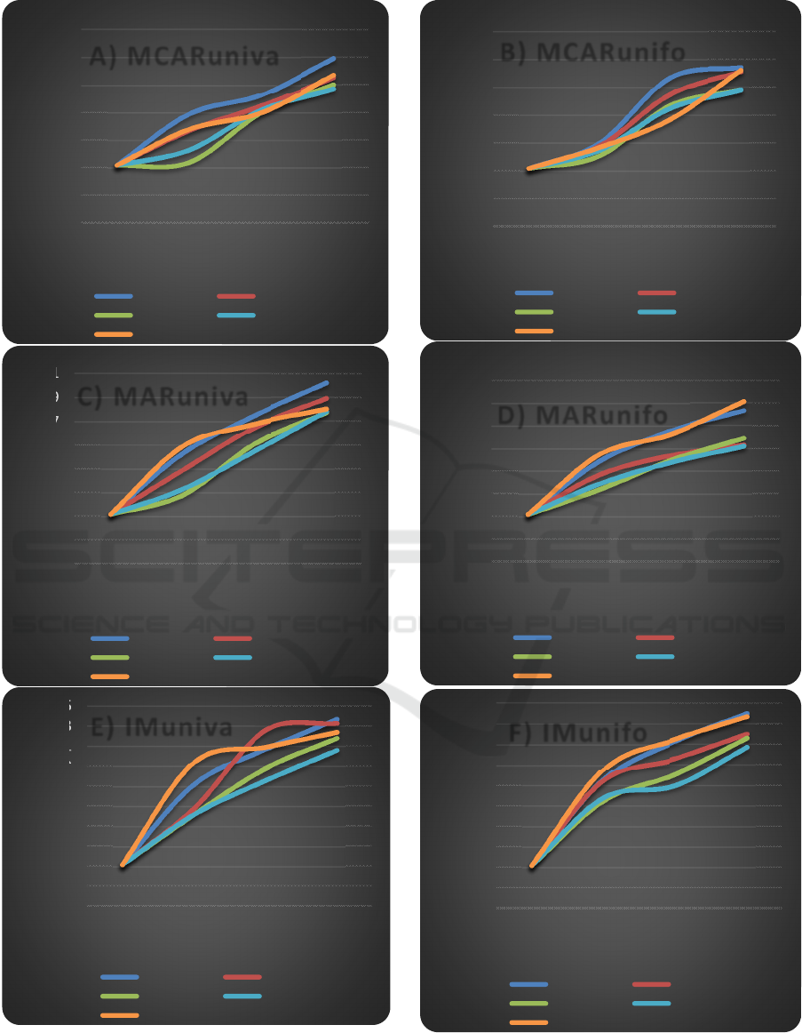
Figure 3: Comparative results of current and new testing methods A) MCARuniva, B) MCARunifo, C) MARuniva, D)

MARunifo, E) IMuniva, F) IMunifo.

0153050

ERROR RATE (%)

REFERENCES

Agresti, A. (1990). Categorical Data Analysis. New York:
John Wiley.
Breiman, L., Friedman, J., Olshen, R., and Stone, C. (1984).
Classification and Regression Trees, Wadsworth.
Cestnik, B., Kononenko, I. and Bratko, I. (1987). Assistant
86 a knowledge-elicitation tool for sophisticated users.
In I. Bratko and N. Lavrac, editors, European Working
Session on Learning – EWSL87. Sigma Press,
Wilmslow, England, 1987.
Cheeseman, P., Kelly, J., Self, M., Stutz, J., Taylor, W., and
Freeman, D. (1988). Bayesian Classification. In
Proceedings of American Association of Artificial
Intelligence (AAAI), Morgan Kaufmann Publishers:
San Meteo, CA, 607-611.
Dempster, A.P., Laird, N.M., and Rubin, D.B. (1977).
Maximum likelihood estimation from incomplete data
via the EM algorithm. Journal of the Royal Statistical
Society, Series B, 39, 1-38.
Hosmer, D.W. and Lameshow, S. (1989). Applied Logistic
Regression. New York: Wiley.
Khosravi, P., Vergari, A., Choi, YJ. and Liang, Y. (2020).
Handling Missing Data in Decision Trees: A
Probabilistic Approach.. https://arxiv.org/pdf/
2006.16341.pdf (Accessed on 16 September 2020)
Lakshminarayan, K., Harp, S.A., and Samad, T. (1999).
Imputation of Missing Data in Industrial Databases.
Applied Intelligence, 11, 259-275.
Little, R.J.A. and Rubin, D.B. (1987). Statistical Analysis
with missing data. New York: Wiley.
Long, J.S. (1998). Regression Models for Categorical and
Limited Dependent Variables. Advanced Quantitative
Techniques in the Social Sciences Number 7. Sage
Publications: Thousand Oaks CA.
McCullagh, P. and Nelder, J.A. (1990). Generalised Linear
Models, 2nd Edition, Chapman and Hall, London,
England.
MULTIPLE IMPUTATION SOFTWARE. Available from
<http:/www.stat.psu.edu/jls/misoftwa.html,
http:/methcenter.psu.edu/EMCOV.html>
Murphy, P. and Aha, D. (1992). UCI Repository of machine
learning databases [Machine-readable data repository].
The University of California, Department of
Information and Computer Science, Irvine, CA.
Quinlan, J.R. (1985). Decision trees and multi-level
attributes. Machine Intelligence. Vol. 11, (Eds.). J.
Hayes and D. Michie. Chichester England: Ellis
Horwood.
Quinlan, JR. (1993). C.4.5: Programs for machine
learning. Los Altos, California: Morgan Kauffman
Publishers, INC.
Rubin, D.B. (1987). Multiple Imputation for Nonresponse
in Surveys. New York: John Wiley and Sons.
Rubin, D.B. (1996). Multiple Imputation After 18+ Years.
Journal of the American Statistical Association, 91,
473-489.
Schafer, J.L. (1997). Analysis of Incomplete Multivariate
Data. Chapman and Hall, London.
Schafer, J.L. AND GRAHAM, J.W. (2002). Missing data:
Our view of the state of the art.
Psychological Methods,
7 (2), 147-177.
Tanner, M.A. AND WONG, W.H. (1987). The Calculation
of Posterior Distributions by Data Augmentation (with
discussion). Journal of the American Statistical
Association, 82, 528-550
Twala, B. (2005). Effective Techniques for Handling
Incomplete Data Using Decision Trees. Unpublished
PhD thesis, Open University, Milton Keynes, UK
Twala, B., Jones, M.C. and Hand, D.J. (2008). Good
methods for coping with missing data in decision trees.
Pattern Recognition Letters, 29, 950-956.
Twala, B and Cartwright, M. (2005). Ensemble Imputation
Methods for Missing Software Engineering Data. 11
th
IEEE Intl. Metrics Symp., Como, Italy, 19-22
September 2005.
Twala, B., Cartwright, M., and Shepperd, M. (2005).
Comparison of Various Methods for Handling
Incomplete Data in Software Engineering Databases.
4
International Symposium on Empirical Software
Engineering, Noosa Heads, Australia, November 2005.
Wu, C.F.J. (1983). On the convergence of the EM
algorithm. The Annals of Statistics, 11, 95-103.
Zhang, X., Yining, W., Jiahui, H., and Chen, Y. (2020).
Predicting Missing Values in Medical Data via
XGBoost Regression. Journal of Healthcare
Information Research. https://doi.org/10.1007/s41666-
020-00077-1 (accessed 16 September 2020).