
Stroke Comparison between Professional Tennis Players and
Amateur Players using Advanced Computer Vision
Lisa Baily
1
, Nghia Truong
2
, Jonathan Lai
3
and Phong Nguyen
2
1
The American School in Japan, 1-1-1 Nomizu, Chofu-shi, Tokyo, Japan
2
Tokyo Techies, Shinbashi 2-16-1, Minato, Tokyo, Japan
3
Tokyo Coding Club, Nishi Azabu 3-24-16, Minato, Tokyo, Japan
Keywords: Pose Estimation, Pose Tracking, Machine Learning, Computer Vision, Euclidean Distance, Tennis, Analysis.
Abstract: In this paper, we created a method to find how professional and amateur tennis serves differ from each other.
We collected videos from online and from our own recordings and turned those videos into frames. From
those frames, we manually selected ones appropriate for our study and ran those through a pose estimation
system, which turned those frames into simple stick figures of the players including all the x and y coordinates
of the player. By normalizing all data, we were able to calculate the Euclidean distance between two compared
players’ joints and analyze their consistency in their serves. Our results from our t-tests showed that there was
a significant difference between the amateur’s consistency and the pro’s consistency and body parts like both
shoulders showed a significant difference.
1 INTRODUCTION
Tennis is a popular competitive and leisure sport that
is played in a one-on-one or two-on-two format. The
sport is largely composed of various “strokes” to keep
the ball in play, such as the forehand and backhand
strokes during a rally and a serve to start the game. Of
those strokes, the serve plays a critical role, as it has
been shown to be one of the two most important shots
along with the return in determining wins
(O'Donoghue and Brown, 2008). It is also a shot with
high variance, with variability in power, ball speed,
accuracy, ball impact location and angular velocities
(Whiteside, et al. 2014, Martin, et al. 2016,). Given
the serve’s significance and variance, amateur players
often observe professional players who compete at
international tournaments like Wimbledon and the
US Open to emulate the form of those top players and
improve their own serve. However, simply watching
them play is not nearly sufficient if the goal is to
understand the real differences between an amateur
and a professional
.
Today, computer vision is a rapidly growing
technology within the broader fields of computer
science and artificial intelligence (Arai and Kapoor
2019; Shavit and Ferens 2019). It is both fairly new
and has a wide range of applications. It can take in
images from videos or photos and provide numerical
evaluations. From those outputs, we can analyze data
more specifically and efficiently and derive
compelling results. Applications of computer vision
in the field of sports include but are not limited to
analysis and evaluation of tennis players (Mukai,
Asano, Hara, 2011), highlight detection (Ren, Jose,
2009) and support decision making (Owens, Harris,
Stennett, 2003).
We propose using computer vision to analyze
tennis shots, and potentially provide amateur players
with the level of specificity and data necessary to help
them improve. Although tennis includes many types
of strokes, we chose to focus on one of the most
important: the serve (O'Donoghue and Brown, 2008).
Although the serve does not require much movement,
as the shot is hit in one stationary location, the way
the serves are hit varies between players, thus making
it difficult to improve just by watching professionals'
play. With a computer vision algorithm, recognizing
what is different and how it is different from
professionals to amateurs will become clearer.
We first split the collected videos into frames and
then used an accurate pose estimation system to
simplify the frames into a stick representation of the
player. After normalizing all data into the same size
and making it comparable, we were able to analyze
the similarities and differences between professional
44
Baily, L., Truong, N., Lai, J. and Nguyen, P.
Stroke Comparison between Professional Tennis Players and Amateur Players using Advanced Computer Vision.
DOI: 10.5220/0010145800440052
In Proceedings of the 8th International Conference on Sport Sciences Research and Technology Support (icSPORTS 2020), pages 44-52
ISBN: 978-989-758-481-7
Copyright
c
2020 by SCITEPRESS – Science and Technology Publications, Lda. All rights reserved

and amateur players, leading to the conclusion that
not only were the patterns between the professionals
and amateurs different, but that specific body part
positioning showed a significant divergence.
2 RELATED WORK
A survey of what has been already published in this
area revealed a range of existing publications that
agreed on the importance of analyzing the serve in
greater detail along with other strokes, but chose to
focus on different components.
In Whiteside et al. (2014), the researchers focused
on the tossing component of the serve and how
important the consistency of it is to the resulting serve.
From their research, they were able to recognize that
while professionals were not consistent in the
horizontal placement of the ball, they were
consistently tossing the ball at the same height. This
paper's main topic was about the serve but it differs
from our paper, as they focused mainly on the toss of
the ball, rather than focusing on the whole serving
motion.
Chow et al. (2007) focused on how the activation
of the muscles varied before and after the impact in
the tennis volley, as many players are concerned
about the after effect, potentially leading to severe
injuries on the wrist. They collected data by placing
electrodes on the players’ bodies. This data
collection was conducted with several controls, such
as the tennis string and racket type. From the EMG
data, they were able to conclude that the oversize
tennis balls “do not significantly increase upper
extremity muscle activation compared to regular size
balls during a tennis volley”. While this paper
focused primarily on volleys and not the serve, the
level of detail it went into showing how even
miniscule changes in one’s form can lead to
drastically different physiological impacts in the
long run reinforced how important our research is
when it comes to a stroke that covers a much wider
range of motion than volleys.
This importance is corroborated by Chow et al.
(2009) which looked into how different types of
serves affect the players' conditions. They included 3
types of serves - flat, topspin, and slice, and examined
how those shots activate the middle and lower trunk
muscles. For each subject, their two highest rated
EMG and kinematic data, which are coordinate data
extracted from their raw videos, were used to analyze
the differences. Even though there were no significant
effects for the serve type on muscle activation, they
found that on average, the largest EMG levels were
observed in the “descending windup or acceleration
phases”. While this does identify certain components
of the serve that hold significant weight, our research
hopes to add data and detail to those components in
order to better understand the angles and stroke
lengths that separate the professional player from the
amateur.
Baily and Nguyen (2018) developed a method to
classify different tennis strokes based on an armband
that measures data from its accelerometer, gyroscope,
quaternion, and EMG. The authors use a supervised
learning model, a Support Vector Machine (SVM), to
determine the correct tennis shot based solely data
from the armband.
3 PROPOSED METHOD
In this section we describe our proposed method we
used to analyze differences in player serves. We first
collected sample serve videos from both amateurs and
professionals from the Internet and our own
recordings. We manually looked through each video
and identified the sets of frames that capture the serve
motion. A pose estimation algorithm is used to
reconstruct the poses of each player appearing in
those frames, and the result is put through a pose
tracking system to label each person with an integer
identifier. We then manually labelled the result with
the player name, ID number, and whether they are
left-handed or not. The labelled pose data is then
normalized to account for the difference in body size,
position in image and left-handedness. Finally, we
calculated the Euclidean distance between the same
limbs in all pairs of serve clips collected and made
observations based on statistical analysis. This is
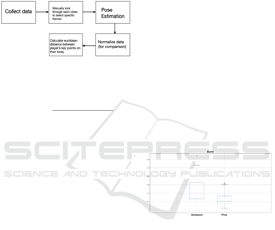
visually represented in Figure 1 below.
Figure 1: Our data pipeline. Black arrows denote manual
steps, and blue arrows denote steps done using computer
programs.
Stroke Comparison between Professional Tennis Players and Amateur Players using Advanced Computer Vision
45

Essential to standardizing our results was the
algorithm used for pose estimation, which has been
one of the major challenges in computer vision since
its introduction. In pose estimation, an algorithm
attempts to determine the positions and the poses of
the humans in a given digital image and helps to
ensure that the data collected is comparable. In this
case, a human pose is defined as a set of points
describing the important body joints. For our problem,
we used the pose estimation algorithm proposed by
Fang, et al. (2017). The framework, named Alpha
Pose, first detects all human locations in an image.
Each location is treated as a single-person image and
fed to a Symmetric Spatial Transformer Network
(Jaderberg et al., 2015) to find the region of interest,
continued to a Single Person Pose Estimator (Newell,
et al., 2016) to estimate the pose in local image and
finally through a Spatial De-Transformer Network to
remap the estimated human pose back to the original
coordinate. The estimated poses are then refined
through the use of parametric Pose Non-Max
Suppression (Fang et al., 2018) to obtain the final
human poses. We used the Alpha Pose authors’
official implementation available on GitHub
(Machine Vision and Intelligence Group, 2017),
which outputs human poses in the Microsoft COCO
(Lin et al., 2015) format
1
.
One of the common concerns in pose estimation
is that in a 2D image, very often some of the important
body joints are not visible. Alpha Pose addresses this
by representing a joint using 3 numbers: x-coordinate,
y-coordinate and a confidence score. The third
number ranges from 0 to 1, with lower values
assigned to less visible joints. Even when a joint is
completely invisible, unless it lies outside of the
image, the model does a good job predicting its
position and assigning a confidence score. Our videos
were chosen so that the main player is always
completely visible in most of the frames, so missing
data wasn’t a big concern. Also, for the sake of
simplicity, we didn’t use the confidence score in our
analysis.
The pose estimation step is repeated for all frames
we wanted to analyze. Note that this analysis is done
in 2 dimensions and not 3, and because we are
analyzing each frame, we compare sets of static poses
of the players, not their overall motion. Since there
can be multiple people in a frame, we needed to
accurately identify the main player in all frames. We
did this by running the pose estimation results
through a pose tracking system, which analyzed the
connectivity of the poses between consecutive frames
1
https://cocodataset.org/#format-data
and assigned an identifier to each human, then
manually reviewed the results and recorded the IDs
of the main players as well as whether they’re left-
handed or not. The tracking system used is Pose Flow
(Xiu, et al, 2018), which is available as an open
source project on GitHub (Machine Vision and
Intelligence Group, 2018). In this system, the pose
estimation result is fed to an optimization framework
to build the association of cross-frame poses and form
pose flows, then to a pose flow non-maximum
suppression to robustly reduce redundant pose flows
and re-link temporal disjoint ones. The result of this
step is a database of poses in MS COCO format with
player name, tracking ID, video link and handedness.
3.1 Data Processing
Serve videos of 4 professionals and 3 amateurs were
used to conduct this research. 3 out of the 4
professionals’ data were collected via the internet and
the rest of the videos were collected on our own. In
the data collection, we used videos including 4~13
serves per player and as a control, all of the videos
were captured from the back angle of the player. With
the videos, we turned them all into frames, thus
making the data manipulation easier. All of the videos
were at 30 frames per second. We manually cut the
frames into smaller sections, with only one full stroke
per section. To keep the frame number per cut equal,
we set a constant of 72 frames. This resulted in each
player having 4~13 serve videos, each consisting of
72 frames, and the number for professionals and
amateurs were roughly equivalent, which makes the
comparison more accurate. To further simplify and
make the analysis accurate, we selected 21 frames
from those 72 frames, including the contact point of
the serve and 10 frames before and after. We selected
those specific frames because the time at which a
player takes before and after their contact point of the
ball during a serve is different and only selecting
frames around the contact point reduces variation
between players during analysis.
In Figure 2, the image highlighted in yellow is the
“contact point” frame, which is the point at which the
player makes contact with the ball at the maximum
height. By adding on 10 frames before and after, the
images capture the serve motion around the ball hit of
the serve for a total of 21 frames.
icSPORTS 2020 - 8th International Conference on Sport Sciences Research and Technology Support
46
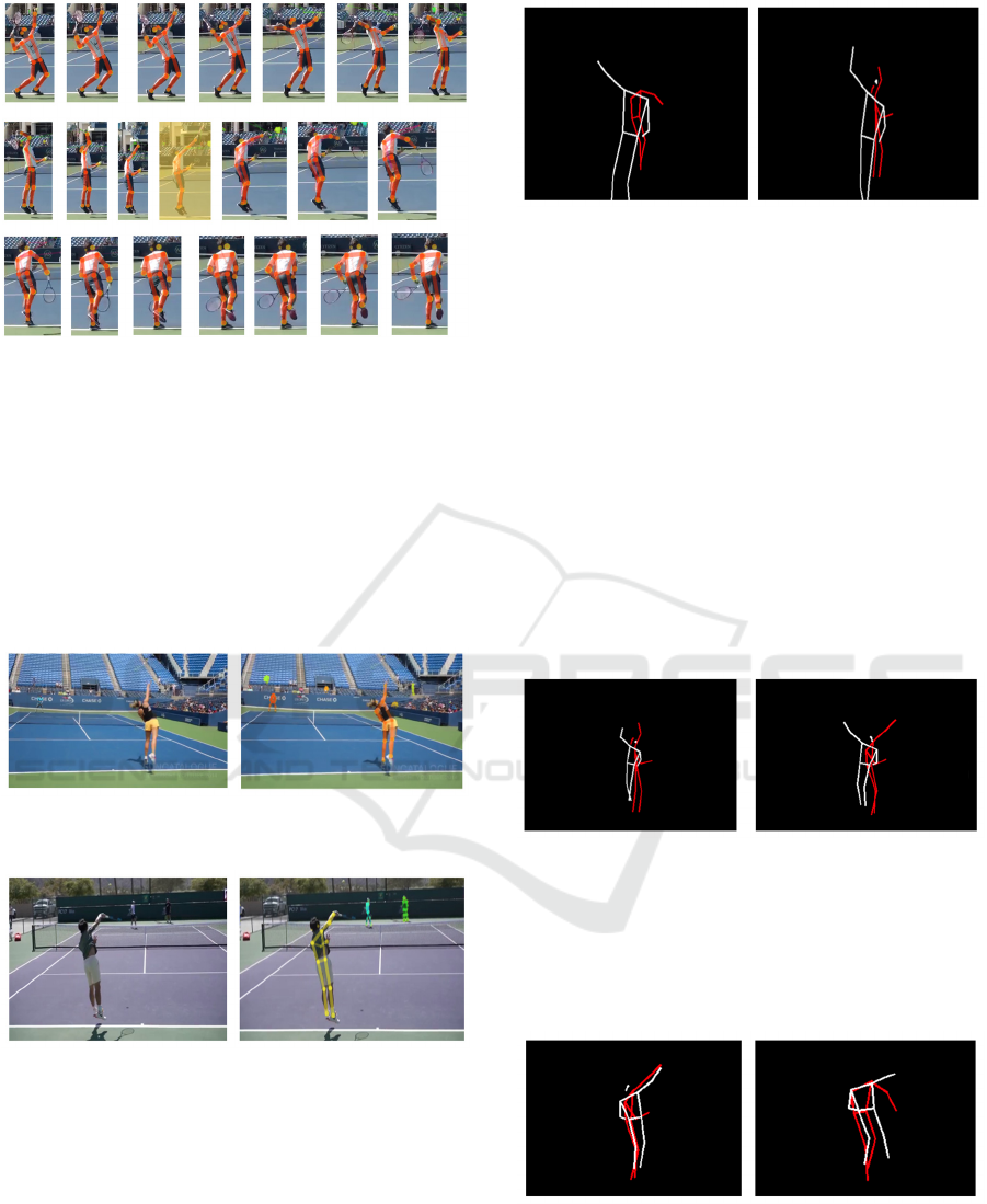
Figure 2: One of the professional’s 21 frames, the contact
point frame and 10 frames before and after.
We then ran the Alpha Pose system on all those
frames we manually collected and the output includes
a stick figure of the players with 17 important points
on the player’s body.
In Figure 3 and 4, we display the output of the
Alpha Pose detection so that one can see the lines and
key points drawn on the player’s body, representing
the simple outline of a human body in one frame.
Figure 3: A female professional player before and after
Alpha Pose detection.
Figure 4: A male professional player before and after Alpha
Pose detection.
Even though all of the videos were taken from the
back of the player, the distance between the player
and the camera varied throughout different videos so
normalizing the scales of the players became essential.
It is clear in Figure 5 that because the scaling is not
applied, the poses do not overlap or match well to
each other.
Figure 5: Comparison of two players (one left-handed
which is the white stick figure and the other right-handed
with the red stick figure) initially without any scaling or
shifting.
We created separate scales for the x axis and the y
axis. To find the right scales for the x coordinates, we
looked through all of the poses’ x coordinates of the
left and right shoulder and found the distance between
them. We repeated this process for the y coordinates,
the left and right hip, and we selected the greatest
values of both the x and y to create the scale. These
scaling factors were then normalized to a set width
and height. After finding the scaling factors we
applied it to all frames and finally shifted the poses,
in order for them to overlap with each other. With the
scaling and shifting, the poses now are comparable,
as shown in Figure 6.
Figure 6: The same players from Figure 5 but scaled and
shifted.
To further improve the comparison, we also
flipped left-handed players so that their data can be
analyzed as well with the right-handed players, which
is displayed in Figure 7 below.
Figure 7: Final output with scaling, shifting, and flipping
(for left-handed players only).
Stroke Comparison between Professional Tennis Players and Amateur Players using Advanced Computer Vision
47
3.2 Comparison
As shown in Figure 8, we first collected the data, then
manually selected the important frames and put those
images through pose estimation.
Figure 8: Flow diagram of the comparison process.
Then with the normalization completed, we
analyzed the data by taking the Euclidean distance
between each of the 17 points on the two players for
all of the frames. We calculated the Euclidean
distance between the same joints of two players by
using the equation
. Each
player has 17 key points detected from the pose
estimation and for each of the key points, the same
point on the other player’s pose estimation was
compared, using the equation above. We repeated this
process for all 17 points and summed up the distances
for us to compare.
To further analyze the differences between
players, we used t-tests to compare the distributions
of the data sets. The t-test data are specifically for the
player’s differences with themselves at their contact
point. Because we were aware that the variances
between each of the players were different, we used a
Welch’s t-test, which can be used on datasets with
varying standard deviations or heteroscedasticity.
Also, we used this type of test because the number of
samples were different for each player.
4 EXPERIMENTAL SETTING
To start off, we gathered videos from several angles
of one player hitting overhead serves. Those videos
were 10 to 30 minutes of a player practicing the serve.
The first couple of serves, around 4 to 5, were ignored
as they showed significant differences with the
following serves and were likely warm-ups, so we
collected 5 to 10 strokes of each player after their
warm-ups. To get a wider variety of players, we
collected data from the Internet where there are plenty
of professional players’ practice videos. In total we
gathered 4 professionals, 3 amateurs, and within those
players, only one player was left-handed. Similar to
the data collection method for the first player, we
ignored the first couple of serves and took the next 5
to 10 serves, making sure that we collected their real
serving style. The point of this research is to compare
pros to pros, amateurs to amateurs, and amateurs to
pros to see whether the consistency amongst those
data sets are significantly different.
5 RESULTS
In this section, we will discuss the results collected
from our data. We first looked at 2 boxplots, side by
side, of the sums of the Euclidean distances between
limbs for amateurs and pros.
The results in Figure 9 clearly show that the
distribution for the amateurs was more spread out
when compared to the pros implying a greater
variance in the data. The median, as well as the
interquartile range of the data, for amateurs are
greater than that for the pros. Knowing that there are
clear distinctions between the distributions of the pros
and amateurs, we looked more closely to where
exactly those differences arise by creating histograms
specific for each player.
Figure 9: Boxplot of the distributions of the sums of the
Euclidean distances between limbs for the amateur and pro
category.
In Figure 10, Figure 11 and Figure 12, the x axis
represents a normalized Euclidean distance between
each of the players, and the y axis represents the
frequency of those distances occurring. Figure 10
compares Amateurs to other Amateurs, Figure 11
compares Professionals to Professionals while Figure
12 compares Professionals to Amateurs. There is a
clear distinction between the distributions of
professionals and amateurs. The professionals’
histograms are more tightly distributed and mostly
skewed to the right, meaning the differences between
their serves were not very large. However, the
histograms of the amateur players have larger ranges
icSPORTS 2020 - 8th International Conference on Sport Sciences Research and Technology Support
48
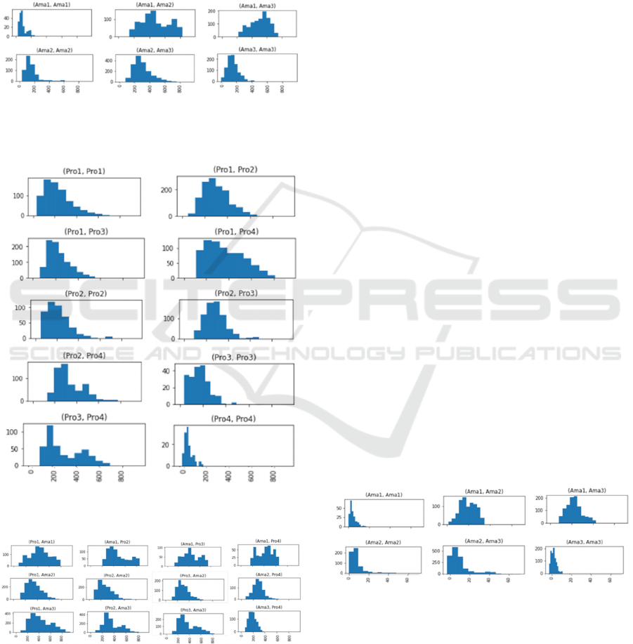
and their distributions are not as skewed compared to
the professionals. This shows how amateur players
were not consistently making similar movements,
thus shifting the distribution towards larger values. In
Figure 12, it shows a histogram with pros and
amateurs being compared to each other. Compared to
Figure 10 and 11, there are no distinct features that
stand out when comparing pros to amateurs.
Figure 10: Histograms of the distributions of the sums of
Euclidean distances between limbs comparing Amateurs to
Amateurs.
Figure 11: Histograms of the distributions of the sums of
Euclidean distances between limbs comparing Pro to Pro.
Figure 12: Histograms of the distributions of the sums of
Euclidean distances between limbs comparing Pro to
Amateur.
Because the histograms only provide qualitative
data, we then used Welch's unequal variance t-test, a
type of statistical analysis to determine whether there
is a significant difference between the means of two
groups. This test showed a similar result when testing
for significant differences between professional and
amateur players.
We conducted a Welch’s t-test between the
professionals’ sums of distances and the amateurs’
sums of distances and the resulting p-value was
0.0036. From this, we were able to conclude that there
is, in fact, a significant difference between the means
of the two groups, the professionals’ sum and the
amateurs’ sum.
To further analyze where exactly those
differences were, we conducted several t-tests, shown
in Table 1, each for the key points on the player’s
body, and found that, while neither of the right wrist
nor left hip were significant, there were significant
differences in the rest of the body points analyzed (all
p-values less than 5%). The p-values for the shoulder
comparisons were most significant. With this, it is
evident that one of the most consistent differences
between amateurs and professionals is in the
shoulders.
In Figures 13, 14, 15, where we plot the
distribution of differences in left shoulder locations
across different player types, it is clear that the
differences between the distributions for the
professional and amateur players are significant. For
instance, Figure 14 shows that Professionals
compared to other different Professionals have a
significantly right skewed distribution while the
Amateurs compared to other different Amateurs
(Figure 13) or Amateurs compared to Professionals
(Figure 15) have a significantly less right skewed
distribution and in some cases are almost
symmetrically distributed.
Figure 13: Histograms of the distributions of the sums of
Euclidean distances between the left shoulder comparing
Amateurs to Amateurs (only left shoulder).
Stroke Comparison between Professional Tennis Players and Amateur Players using Advanced Computer Vision
49
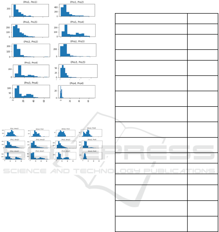
Figure 14: Histograms of the distributions of the sums of
Euclidean distances between the left shoulder comparing
Pro to Pro (only left shoulder).
Figure 15: Histograms of the distributions of the sums of
Euclidean distances between the left shoulder comparing
Amateur to Pro (only left shoulder).
We conducted another test to see if there are clear
distinctions between the distributions of differences
of professional player serves compared to other
professional players and the differences of amateur
player serves compared to other amateur players. In
other words, we are comparing the difference in the
pro distribution versus the amateur distribution.
From this we were able to conclude that those two
groups are, in fact, significantly different from each
other, with respect to intra-group differences, with a
p-value of 2.735 10
. In contrast, there was no
significant difference in amateur distribution to the
distribution of pro vs amateur differences.
Although we only focused on some of the p-value
results, the numbers in Table 1 shows all of our results
and although some values are not significant, others
show a significant value, like the pro-to-pro to pro-to-
amateur.
Table 1: All of the collected p-value results for different
types of distributions.
Compared Distributions P-values
Pro Sum to Amateur Sum
0.0036
Pro Right-Sum to Amateur Right-
Sum
0.0532
Pro Left-Sum to Amateur Left-Sum
0.00463
Pro Upper-Sum to Amateur Upper-
Sum
0.021998
Pro Left-Elbow to Amateur Left-
Elbow
0.02279
Pro Right-Elbow to Amateur Right-
Elbow
0.003554
Pro Right-Shoulder to Amateur
Right-Shoulder
3.729 10
Pro Left-Shoulder to Amateur Left-
Shoulder
1.21 10
Pro Right-Wrist to Amateur Right-
Wrist
0.9789
Pro Left-Wrist to Amateur Left-Wrist
0.0346
Pro Right-Hip to Amateur Right-Hip
2.324 10
Pro Left-Hip to Amateur Left-Hip
0.0857
Pro-to-Pro to Amateur-to-Amateur
2.735
10
Pro-to-Pro to Pro-to-Amateur
3.083
10
Amateur-to-Amateur to Pro-to-
Amateur
0.3798
6 DISCUSSION
In this section, we will discuss some possible
explanations and implications of our results and will
evaluate the strengths and weaknesses of our research.
To start off, not only have we confirmed the
obvious result that professional body movements
during serves are significantly different to amateurs
in terms of consistency. We have also shown that
professionals are more consistent among each other
icSPORTS 2020 - 8th International Conference on Sport Sciences Research and Technology Support
50

as a group then amateurs. Our main result however is
our ability to narrow down the differences to each
limb area and do so with only a simple single
recording of the player without the need for special
set ups. Indeed, nearly half of our analyzed player
videos came from publicly available videos.
Among our limb differences, while most limb
areas showed significant differences from pros to
amateurs, the right wrist and left hip were not
significantly different, in fact the right wrist was
significantly similar. Given that we analyzed serves
frames around the ball contact point, this implies most
players, professional and amateurs alike, can manage
to position their racket to an optimal contact point
with the ball, even if the rest of their body and
footwork is dissimilar or suboptimal. Although, the
left hip and leg is where most players are often taught
to keep their weight during a serve, the p-values seem
to indicate there isn’t a significant difference in how
pros and amateurs position this limb even if there
might be some small variations. This may imply that
most players, even amateurs, reach a good level of
consistency with this limb.
Our findings are definitely informative to tennis
players. This gives players points they can focus on
improving and points where they may not need to
spend as much effort, rather than watching
professionals and not knowing where to pay attention.
It allows amateur players to have an objective
understanding in their performance consistency,
compared to other professionals and other amateur
players. This data can be helpful to tennis coaches, as
it gives them a focus point in their lessons. Our data
is applicable to a wide range of players in a wide
range of situations because of our normalization
methods we applied on all stroke data and the
minimal requirements for the analysis videos, limited
to only their shooting angle, without need for special
preparation.
However, the drawbacks are that we had to
manually select the 21 frames (1 contact point frame,
10 frames before and after), which we would ideally
like to automate. Additionally, because we looked
into each video by frames, this means that we only
considered a series of static poses, not a time
evolution and that is one limitation our research has.
The static poses are adequate enough for the research
but it also means that the overall flow of the strokes
are disregarded, meaning we could have been
overlooking important parts regarding the overall
movements of the player’s strokes. Another weak
point of our research is that our analysis was only in
2 dimensions, not 3 dimensions. This is a limitation
as even though the player’s movements are in 3
dimensions, we are only looking at the x and y
coordinates. However, because we are focusing on
analyzing players from only a single camera angle, 3-
dimensional analysis poses significant challenges that
require dedicated testing with a multiple camera setup
to adequately address. Finally, we conducted our
research with only 7 athletes, which included 3
amateur and 4 professional players, and that is
considerably a low number of data points. In our
future work, the research can be further developed by
collecting more data for different players to ensure
more diversity in our collection.
7 CONCLUSIONS
In this paper, we collected videos of both amateur and
professional tennis players, and through the use of
pose estimation and tracking, we were able to
simplify frame images from videos into stick figures.
With the given data, we analyzed the differences
between players’ key points on their body, such as
their shoulders and elbows. This led us to understand
better how the consistency between pros and
amateurs differ and where the biggest differences lie.
For example, in our P-value table, we found
significant differences in both shoulders while the
right wrist showed little difference between
professionals and amateurs. In future works, we look
to further identify differences between professionals
and amateurs looking at differences in limb position
and also body dynamics. Through our t-tests, we
were able to conclude that the distributions of overall
Euclidean distance between limbs as well as specific
limbs such as the left shoulder, right shoulder, and
right hip, for professionals and amateurs were
significantly different.
REFERENCES
Arai, K., Kapoor, S. 2019. Advances in Computer Vision,
Proceedings of the 2019 Computer Vision Conference
(CVC), Volume 1. Springer.
Baily, L., Nguyen, P., 2018. Tennis Stroke Classification
using Myo Armband. The 1
st
International Young
Researchers Conference, 2018.
Chow, J., Knudson, D., Tillman M., and Andrew, D., 2007.
Pre and postimpact muscle activation in the tennis
volley: effects of ball speed, ball size and side of the
body. British Journal of Sports Medicine.
Chow, J., Park, S., Tillman, M. 2009. Lower trunk
kinematics and muscle activity during different types of
tennis serves. BMC Sports Sci Med Rehabil 1, 24
Stroke Comparison between Professional Tennis Players and Amateur Players using Advanced Computer Vision
51

Fang, H.-S., Xie, S., Tai, Y.-W., Lu, C., 2017. RMPE:
Regional multi-person pose estimation, in International
Conference on Computer Vision (ICCV).
Jaderberg, M., Simonyan, K., Zisserman, A., Kavukcuoglu,
K., 2015. Spatial transformer networks. In Conference
on Neural Information Processing Systems (NIPS),
pages 2017–2025.
Lin, T.-Y., Maire, M., Belongie, S., Bourdev, L., Girshick,
R., Hays, J., Perona, P., Ramanan, D., Zitnick, C. L.,
Dollár, P., 2015. Microsoft COCO: Common objects in
context, in International Conference on Computer
Vision (ICCV).
Machine Vision and Intelligence Group at Shanghai Jiao
Tong University, 2017. AlphaPose. GitHub repository.
https://github.com/MVIG-SJTU/AlphaPose
Machine Vision and Intelligence Group at Shanghai Jiao
Tong University, 2018. PoseFlow. GitHub repository.
https://github.com/YuliangXiu/PoseFlow
Martin C, Bideau B, Delamarche P, Kulpa R, 2016.
Influence of a Prolonged Tennis Match Play on Serve
Biomechanics. PLoS ONE 11(8): e0159979.
Mukai, R., Asano, T. and Hara, H., 2011. Analysis and
Evaluation of Tennis Plays by Computer Vision, 2011
International Conference on Mechatronics and
Automation (ICMA), pages 784–788
Newell, A., Yang, K., and Deng, J., 2016. Stacked
hourglass networks for human pose estimation. In arXiv
preprint arXiv:1603.06937
O'Donoghue, P., Brown, E., 2008. The Importance of
Service in Grand Slam Singles Tennis. International
Journal of Performance Analysis in Sport. 8. 70-78.
Owens, N., Harris, C., Stennett, C., 2003. Hawk-eye tennis
system, International Conference on Visual
Information Engineering.
Ren, R., Jose J. M., 2009. General highlight detection in
sport videos, ACM Multimedia Modeling 2009, pages
27-38
Shavit, Y., Ferens, R., 2019. Introduction to Camera Pose
Estimation with Deep Learning. In arXiv preprint
arXiv:1907.05272.
Whiteside, D., Giblin, G., Reid, M., 2014. Redefining
Spatial Consistency in the Ball Toss of the Professional
Female Tennis Serve. 32 International Conference of
Biomechanics in Sports.
Xiu, Y., Li, J., Wang, H., Fang, Y., Lu, C., 2018. Pose Flow:
Efficient online pose tracking. In arXiv preprint
arXiv:1802.00977.
icSPORTS 2020 - 8th International Conference on Sport Sciences Research and Technology Support
52
