Towards Optical Flow Ego-motion Compensation for Moving Object
Segmentation
Ren
´
ata Nagyn
´
e Elek
1,2 a
, Art
´
ur I. K
´
aroly
1,2 b
, Tam
´
as Haidegger
1,3 c
and P
´
eter Galambos
1,3 d
1
Antal Bejczy Center for Intelligent Robotics, Univ. Research and Innovation Center,
´
Obuda University, Budapest, Hungary
2
Doctoral School of Applied Informatics and Applied Mathematics,
´
Obuda University, Budapest, Hungary
3
John von Neumann Faculty of Informatics,
´
Obuda University, Budapest, Hungary
Keywords:
Optical Flow, Ego-motion, Velocity Compensation, Moving Object Segmentation, Robotics.
Abstract:
Optical flow is an established tool for motion detection in the visual scene. While optical flow algorithms
usually provide accurate results, they can not make a difference between image-space displacements origi-
nated from moving objects in the space and the ego-motion of the moving viewpoint. In the case of optical
flow-based moving object segmentation, camera ego-motion compensation is essential. Hereby, we show the
preliminary results of a moving viewpoint optical flow ego-motion filtering method, using two dimensional op-
tical flow, image depth information and the camera holder robot arm’s state of motion. We tested its accuracy
through physical experiments, where the camera was fixed on a robot arm, and a test object was attached onto
an other robot arm. The test object and the camera were moved relative to each other along given trajectories
in different scenarios. We validated our method for optical flow background filtering, which showed 94.88%
mean accuracy in the different test cases. Furthermore, we tested the proposed algorithm for moving object
state of motion estimation, which showed high accuracy in the case of translational and rotational movements
without depth variation, but lower accuracy, when the relative motion produced change in depth, or the camera
and the moving object move in the same directions. The proposed method with future work including outlier
filtering and optimisation could become useful in various robot navigation applications and optical flow-based
computer vision problems.
1 INTRODUCTION
Moving object segmentation in computer vision is
a principal problem including, but not limited to
content-based video coding (Shao-Yi Chien et al.,
2002), autonomous driving (Siam et al., 2017),
mobile robot navigation and collision avoidance
(Talukder et al., 2003) as well as healthcare technolo-
gies (Garc
´
ıa-Peraza-Herrera et al., 2017), where most
recent Deep Learning algorithms cannot provide fast
enough solutions (K
´
aroly et al., 2018). Optical flow
– which is a pattern of motion of objects in a visual
scene – and moving objects in the space are neces-
sarily related, thus optical flow-based moving object
segmentation is an obvious approach. A recent study
(Cheng et al., 2017) investigates an end-to-end train-
a
https://orcid.org/0000-0002-3030-254X
b
https://orcid.org/0000-0002-2902-7253
c
https://orcid.org/0000-0003-1402-1139
d
https://orcid.org/0000-0002-2319-0551
able network for predicting pixel-wise object segmen-
tation and optical flow method. Background subtrac-
tion can be a pre-filter for optical flow applications as
well. In (S
´
anchez-Ferreira et al., 2012), a Field Pro-
grammable Gate Arrays (FPGA) based background
filter can be found for motion detection. However, op-
tical flow-based moving object segmentation can be
a much more complex problem, if the viewpoint is
moving as well; optical flow techniques cannot make
a difference between motion originated from moving
objects in the space and from the self-motion of a
moving camera. The motion of the viewpoint – called
’self-motion’, or ’ego-motion’ – has to be extracted
from the optical flow vector field to detect moving
objects in the space. The two main approaches for
ego-motion filtering is the usage of the viewpoint’s
state of motion, or subtract the background motion
without this prior knowledge. An early paper pro-
posed an ego-motion filter method with robust recog-
nition of moving objects without any knowledge of
the viewpoint state of motion; however, this solu-
114
Elek, R., Károly, A., Haidegger, T. and Galambos, P.
Towards Optical Flow Ego-motion Compensation for Moving Object Segmentation.
DOI: 10.5220/0010136301140120
In Proceedings of the International Conference on Robotics, Computer Vision and Intelligent Systems (ROBOVIS 2020), pages 114-120
ISBN: 978-989-758-479-4
Copyright
c
 2020 by SCITEPRESS – Science and Technology Publications, Lda. All rights reserved

tion can only subtract translational motion (Talukder
et al., 2003), which was extended by a solution for
ego-motion filtering by measuring the likelihood that
a tracked image feature corresponds to a moving 3D
point; the monocular solution uses the prior state of
motion (Klappstein et al., 2009). In (Roberts et al.,
2009) an other approach can be found, where refer-
ence state of motion is not used; they exploited prob-
abilistic linear subspace constraints on the flow to fil-
ter the ego-motion. Bloesch et al. proposed a method
which fuses optical flow and inertial measurements
for ego-motion estimation (Bloesch et al., 2014). An
analogous problem has been resolved in Computer-
Integrated Surgery by (Haidegger, 2019).
In this paper, we propose an optical flow ego-
motion filtering method for background motion com-
pensation in the case of a moving viewpoint, with ac-
cess to the robot’s state of motion and depth informa-
tion. The result is the optical flow vector field with-
out the flow vectors originated from the movement of
the viewpoint. The proposed method can provide the
velocity of the moving obstacle in the space. The
ego-motion filtered optical flow vector field can be
the input for object segmentation techniques (K
´
aroly
et al., 2019), self-driving technologies or other, not
necessarily mobile robot-based problem approaches,
such as Robot-Assisted Minimally Invasive Surgery
(Garc
´
ıa-Peraza-Herrera et al., 2017). In our method
to calculate the ego-motion filtered flow vectors, the
following pieces information are necessary:
• Optical flow matrix;
• Depth information of the scene;
• Camera intrinsic parameters;
• Reference (moving robot) state of motion.
The paper is structured as follows: Section 2 in-
troduces the software and hardware environment used
throughout the study, the applied optical flow tech-
niques, the proposed method and the test arrange-
ment. Section 3 overviews the results of the exper-
iments and shows the advantages and drawbacks of
the introduced method. Section 4 draws conclusion
and discusses the planned future work.
2 MATERIALS AND METHODS
2.1 Software and Hardware
Environment
All of the program codes were implemented in Python
3 programming language in addition with OpenCV 4
computer vision library. To provide the grayscale im-
age data and depth information, an Intel RealSense
SR300 depth camera was used. SR300 implements a
short range, coded light 3D imaging system (Zabatani
et al., 2019). Intel RealSense supports Python pro-
gramming with pyrealsense library. The description
of the robotic test setup can be found in Section 2.4.
2.2 Optical Flow
Optical flow is a pattern of motion of objects in a vi-
sual scene caused by the relative motion between the
observer and the scene (Sun et al., 2010). Optical
flow refers to the motion in the visual field based on
pixel intensities, and however, this motion not neces-
sarily refers to the motion in the real world, in most
of the cases it is a robust tool for motion detection.
There are different approaches for computing the op-
tical flow, such as Horn-Schunck and Lucas-Kanade
methods (Bruhn et al., 2005). The fundamental as-
sumption in optical flow is that the intensity of the
pixels is not changing during the motion. Neverthe-
less, beyond this assumption, the optical flow equa-
tion is still under-determined; thus, the different ap-
proaches use further restrictions, e.g., that the inten-
sity of the local neighbors of pixels changes simi-
larly. The two main categories of optical flow tech-
niques are dense and sparse algorithms. Dense op-
tical flow techniques calculate optical flow for all
pixels, sparse techniques calculate the flow just for
some pixels (special features, such as corners, edges).
Based on the different approaches, dense optical flow
is more accurate, but naturally, it needs more com-
putational capacity. For this work, the chosen tech-
nique was a dense optical flow method, the Farneback
optical flow. The Farneback method has high ac-
curacy, and for ego-motion filter testing, it is use-
ful to examine all of the pixels in the image. The
Farneback algorithm is a two-frame optical flow cal-
culation technique that uses polynomial expansion,
where a polynomial approximates the neighborhood
of the image pixels. Quadratic polynomials give the
local signal model represented in a local coordinate
system (Farneb
¨
ack, 2003).
2.3 Optical Flow Ego-motion
Compensation Method
In this section, we will overview the proposed opti-
cal flow ego-motion filter method. Since Farneback’s
method is a classic approach for optical flow equation
solving, introducing the technique in detail is not in
focus in this paper. In the following equations, we
will show the method through only one pixel. For
Towards Optical Flow Ego-motion Compensation for Moving Object Segmentation
115

ego-motion filtering, it is necessary to take these steps
for the whole image.
Based on the optical flow algorithm, we can get the
pixel displacements; then the current pixel locations
can be calculated:
dx = x
i
− x
i−1
(1)
dy = y
i
− y
i−1
(2)
Where x
i
, y
i
is the current pixel location, and x
i−1
, y
i−1
is the previous pixel location. The pixel to camera
coordinate method can be calculated from the camera
coordinate to pixel perspective projection equation:


x
i
y
i
1


=



f
s
x
0 o
x
0
0
f
s
y
o
y
0
0 0 1 0






X
i
Y
i
Z
i
1



(3)
where x
i
, y
i
are the pixel coordinates, the intrinsic
parameters are the focal length (f), principal point
(o
x
, o
y
), and pixel size (s
x
, s
y
). X
i
, Y
i
, Z
i
are the camera
coordinates. Expand the perspective projection equa-
tion we can get the following equations:
x
i
=
1
s
x
f
X
i
Z
i
+ o
x
(4)
y
i
=
1
s
y
f
Y
i
Z
i
+ o
y
(5)
since we have the depth information (Z
i
), we can cal-
culate the point coordinates:
X
i
=
s
x
f
Z
i
(x
i
− o
x
) (6)
Y
i
=
s
y
f
Z
i
(y
i
− o
v
). (7)
The x
i−1
, y
i−1
previous pixels have to be deprojected
with the same method (Equations 6, 7). From the
current (X
i
, Y
i
Z
i
) and previous camera coordinates
(X
i−1
, Y
i
1
, Z
i−1
) and the elapsed time (dt) we can cal-
culate the current optical velocity (v
i,opt
):
v
i,opt
=
(X
i
, Y
i
, Z
i
) − (X
i−1
, Y
i−1
, Z
i−1
)
dt
. (8)
To compensate the ego-motion, the reference velocity
has to be subtracted from the optical velocity. For this,
we have to transform the camera coordinates with
the transformation matrix originated from the robot’s
translation and rotation to get the actual camera coor-
dinates:



X
i,sel f
Y
i,sel f
Z
i,sel f
1



=

R
cam
2,1
t
cam
2,1
0 0 0 1




X
i−1
Y
i−1
Z
i−1
1



(9)
where (X
i,sel f
, Y
i,sel f
, Z
i,sel f
) are the current camera
coordinates originated from the viewpoint’s motion.
After that, the reference velocity can be calculated:
v
i,sel f
=
(X
i,sel f
, Y
i,sel f
, Z
i,sel f
) − (X
i−1
, Y
i
1
, Z
i−1
)
dt
.
(10)
From v
i,opt
and the reference velocity v
i,sel f
the fil-
tered optical flow can be estimated:
v
i, f iltered
= v
i,opt
− v
i,sel f
(11)
where v
i, f iltered
is the 3D ego-motion filtered optical
flow.
2.4 The Experimental Setup
To test the accuracy of the implemented optical flow
ego-motion filtering method, two Universal Robots
UR5 manipulators were used (Kebria et al., 2016)
(Fig. 1). The test scenarios were set up under the fol-
lowing conditions:
• The first robot arm holds the camera attached to
the last link (known transformation to the robot’s
base coordinate system);
• The second robot holds a test object attached to
the last link (known transformation to the robot’s
base coordinate system);
• Known transformation between the two robots’
base frame.
Both of the robot arms moved on predefined tra-
jectories with synchronized logging of their motion
states and the camera frames. The standard Hough
transform was employed for the test object segmenta-
tion (Mukhopadhyay and Chaudhuri, 2015).
3 RESULTS
For testing purposes, six different scenarios were set
up, where the object holder and the camera holder arm
moved under different conditions (Fig. 1). The de-
tails of the scenarios can be found in Table 1, where
every value is shown in the camera coordinate sys-
tem. The camera coordinate system is right-handed
with the Y-axis pointing down, X-axis pointing right,
and Z-axis pointing away from the camera. During
the motions, the velocities were constant. In Table 1
v
cam
linear
is the linear velocity of the camera, v
cam
angular
is the angular velocity of the camera, and v
ob j
linear
is
the test object’s linear velocity. ”Distance” is the dis-
tance between the camera and the moving object at
the start point of the recording. In Scenarios 1,2 and
ROBOVIS 2020 - International Conference on Robotics, Computer Vision and Intelligent Systems
116

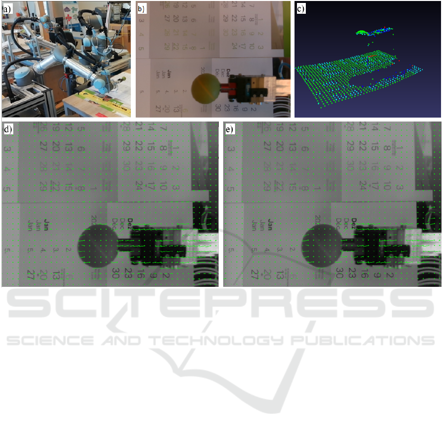
Figure 1: Optical flow ego-motion compensation method test setup and results. A) Test setup with UR5 robots: the robot
on the left holds the test object, the robot on the right holds the depth camera. In the illustrated case, both arms moved in
X direction in front of each other (Scenario 1); b) test setup in the camera scene; c) point cloud of the deprojected pixels
before filtering; green color means minimum velocity in x direction, dark blue means maximum velocity in x direction based
on optical flow; e) two dimensional optical flow before ego-motion compensation; e) two dimensional optical flow after
ego-motion compensation.
3 there were only translational movements performed
by the camera and the test object. In Scenario 4,5, and
6, the camera performed rotational movement. We
tested the accuracy with different velocities and dif-
ferent distances.
The main goal of this research was to filter the
robot’s motion from the optical flow vector field. To
test the accuracy of the background filtering, we cal-
culated the ratio of the number of filtered pixels and
the number of moving pixels before the filtering in
the background. The background was extracted based
on the depth information. These calculations showed
promising results for all of the experiments (best case
scenario showed 99.6% accuracy; the worst case was
89.3%, Table 3). Based on these findings, we can con-
clude that the proposed method shows high accuracy
results of ego-motion background filtering. Another
approach to measuring the accuracy of ego-motion fil-
tering is to compare the segmented moving object’s
state of motion after the filtering to the object’s ref-
erence state of motion. For this, we segmented the
test object on the pre-filtered image and compared the
calculated velocity with the test object holder arm’s
velocity. The results can be found in Table 2, where
the notions are the same as in Table 1. Mean, standard
deviation (Std) and Mean Absolute Error (MAE) were
calculated from a set of frames. We got very accurate
results in the case of Scenario 1, 2, and 4, and low ac-
curacy in the case of Scenario 2, 5, and 6 (Fig. 2). The
results suggest that movements without depth chang-
ing (in our case translation in X and Y direction and
rotation around Z-axis) can be easier to filter to the
algorithm, but movements including depth changing
(in our case rotation around Y-axis and translation in
X, Y and Z directions) can be more complex to filter.
Higher velocity differences between objects of inter-
est and the camera can provide more accurate results.
On the other hand, the relative movement direction
between the object and the camera can be significant
as well: if they are moving in the same direction, it
is harder to extract ego-motion (Scenarios 5 and 6).
Based on these findings, we can conclude that in our
optical flow ego-motion filter solution an ideal case
is where the robot’s and the moving object’s state of
Towards Optical Flow Ego-motion Compensation for Moving Object Segmentation
117

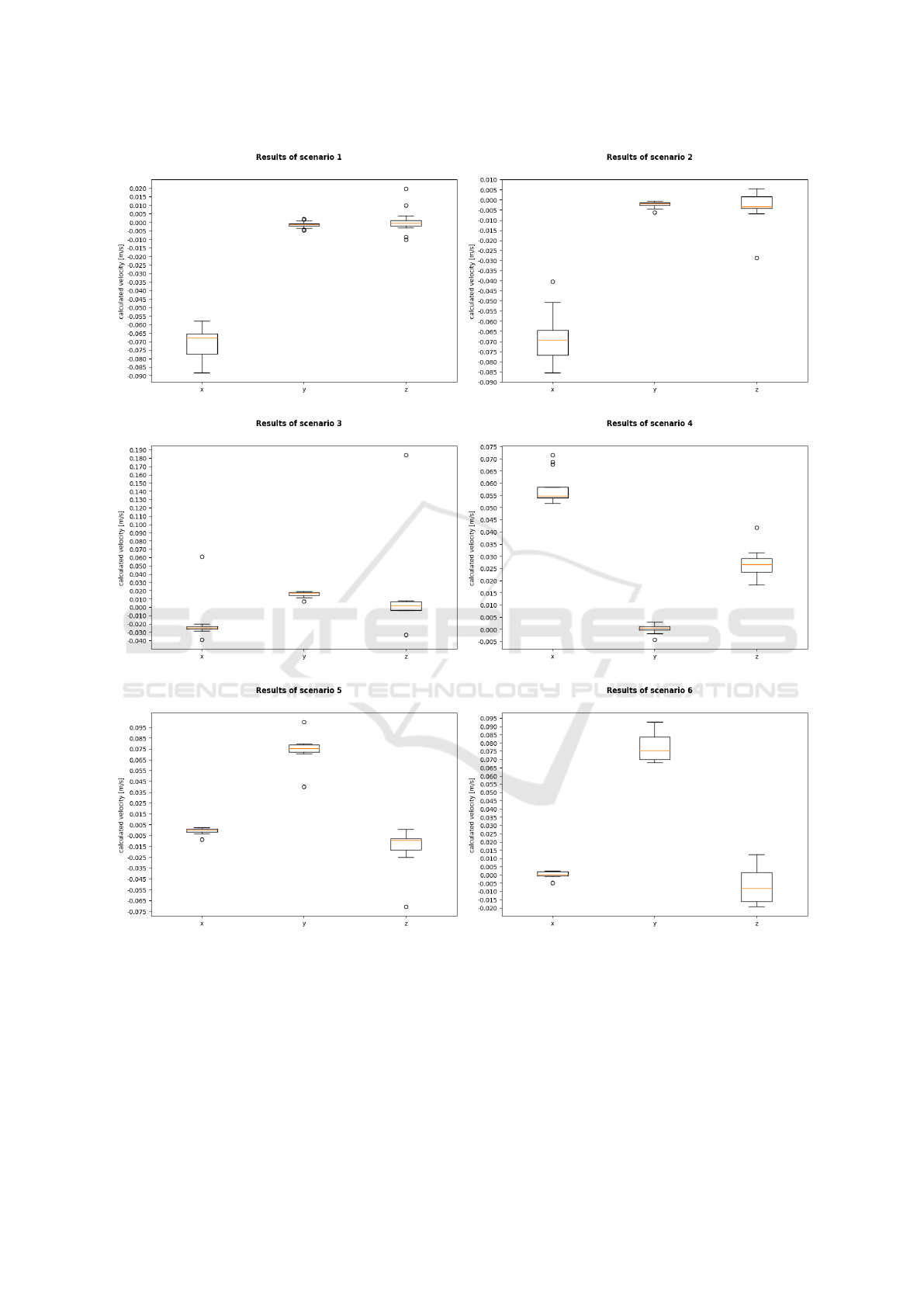
Figure 2: State of motion estimation boxplot results by frames after optical flow ego-motion filtering in the different scenarios.
motion is significantly differs on the projected image
plane. It is important to note that the performance
of the method highly depends on the accuracy of the
depth information provided by a depth sensor.
4 CONCLUSIONS AND FUTURE
WORK
In this paper, we introduced the results of a prelim-
inary study of an optical flow ego-motion filtering
method. It is based on two-dimensional Farneback
ROBOVIS 2020 - International Conference on Robotics, Computer Vision and Intelligent Systems
118

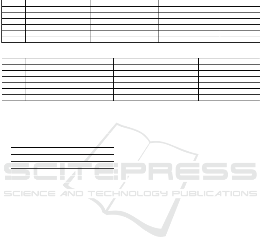
Table 1: Scenario settings for testing the proposed method.
Scen.# v
cam
l inear
((x,y,z), [m/s]) v
cam
angul ar
((x,y,z), [rad/s]) v
ob j
l inear
((x,y,z), [m/s]) Distance ([m])
1 (0.072, 0, 0) (0, 0, 0) (-0.072, 0, 0) 0.33
2 (0.072, 0, 0) (0, 0, 0) (-0.069, 0.012, 0) 0.33
3 (0.021, 0.018, 0.015) (0, 0, 0) (-0.033, 0, 0) 0.36
4 (0, 0, 0) (0, 0, 0.5445) (0.057, 0, 0) 0.23
5 (0, 0, 0) (1.617, 0, 0) (0, -0.057, 0) 0.24
6 (0, 0, 0) (1.617, 0, 0) (0, -0.057, 0) 0.35
Table 2: Results of optical flow ego-motion filtering and moving object state of motion estimation.
Scen.# Mean of calc. v
ob j
l inear
((x,y,z), [m/s]) Std of calc. v
ob j
l inear
((x,y,z), [m/s]) MAE ((x,y,z), [m/s])
1 (-0.071, -0.001, 0) (0.009, 0.002, 0.006) (0.001, -0.001, 0)
2 (-0.068, 0.002, 0.004) (0.013, 0002, 0.009) (0.001, -0.01, 0.004)
3 (-0.016, 0.015, 0.020) (0.029, 0.004, 0.06) (0.017, 0.015, 0.020)
4 (0.058, 0, 0.027) (0.007, 0.002, 0.005) (0.001, 0, 0.027)
5 (-0.001, 0.074, -0.02) (0.004, 0.016, 0.002) (-0.001, 0.131, -0.02)
6 (0, 0.078, -0.006) (0.0023, 0.009, 0.011) (0, 0.135, -0.006)
Table 3: Results of optical flow ego-motion filtering accu-
racy.
Scen.# Background filter accuracy [%]
1 98.0
2 98.5
3 99.6
4 89.3
5 93.9
6 90.0
dense optical flow and image depth information. The
camera’s translational and rotational movement refer-
ence frame is known in our approach. The accuracy
was tested with a moving test object, whose state of
motion is also known. The background filter results
showed very high accuracy – 94.88% on average, in
the different test scenarios). The accuracy of mov-
ing object state of motion estimation was high without
camera depth changing, but low if the camera’s depth
was changing, or the camera and the moving object
are moving in the same direction.
Our most crucial future work is the optimization
of the method and the implementation of outlier filter-
ing. Moreover, our method is planned to be used as a
pre-filter for neural network-based optical flow mov-
ing object segmentation. It may be employed inde-
pendently not only for mobile robot applications, but
also for other robotic problems, where the optical flow
is applied, such as in the case of Robot-Assisted Mini-
mally Invasive Surgery skill assessment (Nagyn
´
e Elek
and Haidegger, 2019).
ACKNOWLEDGEMENTS
Authors thankfully acknowledge the financial support
of this work by the Hungarian State and the European
Union under the EFOP-3.6.1-16-2016-00010 and
GINOP-2.2.1-15-2017-00073 projects. T. Haidegger
and R. Nagyn
´
e Elek are supported through the New
National Excellence Program of the Ministry of Hu-
man Capacities. T. Haidegger is a Bolyai Fellow of
the Hungarian Academy of Sciences. Authors thank
S
´
andor Tarsoly for helping with the UR5 program-
ming.
REFERENCES
Bloesch, M., Omari, S., Fankhauser, P., Sommer, H.,
Gehring, C., Hwangbo, J., Hoepflinger, M. A., Hutter,
M., and Siegwart, R. (2014). Fusion of optical flow
and inertial measurements for robust egomotion esti-
mation. In 2014 IEEE/RSJ International Conference
on Intelligent Robots and Systems, pages 3102–3107.
Bruhn, A., Weickert, J., and Schn
¨
orr, C. (2005). Lu-
cas/Kanade Meets Horn/Schunck: Combining Local
and Global Optic Flow Methods. International Jour-
nal of Computer Vision, 61(3):211–231.
Cheng, J., Tsai, Y.-H., Wang, S., and Yang, M.-H. (2017).
SegFlow: Joint Learning for Video Object Segmenta-
tion and Optical Flow. In Proceedings of the IEEE
International Conference on Computer Vision, pages
686–695.
Farneb
¨
ack, G. (2003). Two-Frame Motion Estimation
Based on Polynomial Expansion. In Goos, G., Hart-
manis, J., van Leeuwen, J., Bigun, J., and Gustavsson,
T., editors, Image Analysis, volume 2749, pages 363–
370. Springer Berlin Heidelberg, Berlin, Heidelberg.
Towards Optical Flow Ego-motion Compensation for Moving Object Segmentation
119

Garc
´
ıa-Peraza-Herrera, L. C., Li, W., Fidon, L., Gruijthui-
jsen, C., Devreker, A., Attilakos, G., Deprest, J.,
Poorten, E. V., Stoyanov, D., Vercauteren, T., and
Ourselin, S. (2017). ToolNet: Holistically-nested
real-time segmentation of robotic surgical tools. In
2017 IEEE/RSJ International Conference on Intelli-
gent Robots and Systems (IROS), pages 5717–5722.
Haidegger, T. (2019). Probabilistic method to improve
the accuracy of computer-integrated surgical systems.
ACTA POLYTECHNICA HUNGARICA: JOURNAL
OF APPLIED SCIENCES, 16(8):119–140.
K
´
aroly, A. I., Elek, R. N., Haidegger, T., Sz
´
ell, K., and
Galambos, P. (2019). Optical flow-based segmenta-
tion of moving objects for mobile robot navigation us-
ing pre-trained deep learning models*. In 2019 IEEE
International Conference on Systems, Man and Cy-
bernetics (SMC), pages 3080–3086.
K
´
aroly, A. I., Full
´
er, R., and Galambos, P. (2018). Unsuper-
vised clustering for deep learning: A tutorial survey.
Acta Polytechnica Hungarica, 15(8):29–53.
Kebria, P. M., Al-wais, S., Abdi, H., and Nahavandi, S.
(2016). Kinematic and dynamic modelling of UR5
manipulator. In 2016 IEEE International Confer-
ence on Systems, Man, and Cybernetics (SMC), pages
004229–004234.
Klappstein, J., Vaudrey, T., Rabe, C., Wedel, A., and Klette,
R. (2009). Moving Object Segmentation Using Op-
tical Flow and Depth Information. In Wada, T.,
Huang, F., and Lin, S., editors, Advances in Image and
Video Technology, Lecture Notes in Computer Sci-
ence, pages 611–623, Berlin, Heidelberg. Springer.
Mukhopadhyay, P. and Chaudhuri, B. B. (2015). A survey
of Hough Transform. Pattern Recognition, 48(3):993–
1010.
Nagyn
´
e Elek, R. and Haidegger, T. (2019). Robot-assisted
minimally invasive surgical skill assessment—manual
and automated platforms. Acta Polytechnica Hungar-
ica, 16(8):141–169.
Roberts, R., Potthast, C., and Dellaert, F. (2009). Learning
general optical flow subspaces for egomotion estima-
tion and detection of motion anomalies. In 2009 IEEE
Conference on Computer Vision and Pattern Recogni-
tion, pages 57–64.
S
´
anchez-Ferreira, C., Mori, J. Y., and Llanos, C. H. (2012).
Background subtraction algorithm for moving object
detection in FPGA. In 2012 VIII Southern Conference
on Programmable Logic, pages 1–6.
Shao-Yi Chien, Shyh-Yih Ma, and Liang-Gee Chen (2002).
Efficient moving object segmentation algorithm us-
ing background registration technique. IEEE Trans-
actions on Circuits and Systems for Video Technology,
12(7):577–586.
Siam, M., Mahgoub, H., Zahran, M., Yogamani, S., Jager-
sand, M., and El-Sallab, A. (2017). MODNet: Mov-
ing Object Detection Network with Motion and Ap-
pearance for Autonomous Driving. arXiv:1709.04821
[cs].
Sun, D., Roth, S., and Black, M. J. (2010). Secrets of
optical flow estimation and their principles. In 2010
IEEE Computer Society Conference on Computer Vi-
sion and Pattern Recognition, pages 2432–2439.
Talukder, A., Goldberg, S., Matthies, L., and Ansar, A.
(2003). Real-time detection of moving objects in a
dynamic scene from moving robotic vehicles. In Pro-
ceedings 2003 IEEE/RSJ International Conference on
Intelligent Robots and Systems (IROS 2003) (Cat.
No.03CH37453), volume 2, pages 1308–1313 vol.2.
Zabatani, A., Surazhsky, V., Sperling, E., Ben Moshe, S.,
Menashe, O., Silver, D. H., Karni, T., Bronstein,
A. M., Bronstein, M. M., and Kimmel, R. (2019).
Intel
R
 RealSense
TM
SR300 Coded light depth Cam-
era. IEEE Transactions on Pattern Analysis and Ma-
chine Intelligence, pages 1–1.
ROBOVIS 2020 - International Conference on Robotics, Computer Vision and Intelligent Systems
120