
Completeness Issues in Mobile Crowd-sensing Environments
Souheir Mehanna
1,2
, Zoubida Kedad
1
and Mohamed Chachoua
2
1
DAVID Laboratory, University of Versailles UVSQ, Versailles, France
2
LASTIG Laboratory, University Gustave Eiffel, EIVP, Paris, France
Keywords:
Data Quality, Data Completeness, Sensor Data.
Abstract:
Mobile sensors are being widely used to monitor air quality to quantify human exposure to air pollution. These
sensors are prone to malfunctions, resulting in many data quality issues, which in turn impacts the reliability
of analytical studies. In this work, we address the problem of data quality evaluation in mobile crowd-sensing
environments, and we focus on data completeness. We introduce a multi-dimensional model to represent the
data coming from the sensors in this context and we discuss different facets of data completeness. We propose
quality indicators capturing different facets of completeness along with the corresponding quality metrics. We
provide some experiments showing the usefulness of our proposal.
1 INTRODUCTION
Air pollution is a global concern because of its major
environmental risk and its adverse effect on health.
According to several WHO
1
reports, air pollution is
a factor in the deterioration and worsening of peo-
ple’s health. It is responsible for an increasing number
of deaths and a myriad of damages to ecological and
economic systems, especially in dense urban cities.
Air quality is often described by the WHO as an invis-
ible killer which has been the main driver for more re-
search in the area in the past recent years. The goal is
to better assess air pollution and its impact on health.
This is the context of the Polluscope
2
research project.
The main objective of this project is to employ micro-
sensors, emerging technologies and the development
of an innovative infrastructure for the acquisition and
exploitation of data, in order to assess air pollution
on very fine scales. This approach aims to charac-
terize the adverse effects on health of air pollutants,
on different scales, in both indoor and outdoor envi-
ronments. Polluscope is a multi-disciplinary project
aiming at quantifying the human exposure to air pol-
lutants in the region of
ˆ
Ile-de-France.
One of the main problems that arise in the Pollus-
cope project is the reliability of the chain of acquisi-
tion and processing of spatio-temporal data. Sensors
and micro-sensing units are well known to be faulty
and prone to points of failures. By the time issues are
1
For more information, see https://www.who.int/home.
2
http://polluscope.uvsq.fr
fixed, the sensors may lose significant chunks of data.
Data analysis based on poor quality data leads to ill-
defined indicators. Hence, it is crucial to monitor data
quality along the entire data processing workflow in
order to provide accurate air quality indicators. This
raises the question of how credible the knowledge in-
duced by the measurements generated by these micro-
sensors is. Which in turn raises other questions such
as: how to ensure the quality of the data from micro-
sensors? How to manage the imperfections of this
data? How to deal with missing data?
This work is a contribution towards data qual-
ity monitoring in mobile crowd-sensing environments
(MCS). We focus on completeness issues raised in
this context. We first propose a multi-dimensional
model representing pollution measurement data along
with the relevant analysis dimensions. We then dis-
cuss the use of this model to capture the different un-
derstandings of the completeness of data coming from
mobile sensors. We introduce completeness indica-
tors, their definition and the appropriate evaluation
metrics.
The rest of this paper is organized as follows. Sec-
tion 2 presents a motivating example. Section 3 intro-
duces the proposed multi-dimensional model to rep-
resent data in MCS environments. Section 4 intro-
duces the sensor completeness indicator and proposes
an evaluation metric. Section 5 deals with the spatial
completeness indicator. Section 6 presents the tem-
poral completeness indicator. Section 7 reports the
experiments performed and the results achieved. Sec-
Mehanna, S., Kedad, Z. and Chachoua, M.
Completeness Issues in Mobile Crowd-sensing Environments.
DOI: 10.5220/0010136201290138
In Proceedings of the 16th International Conference on Web Information Systems and Technologies (WEBIST 2020), pages 129-138
ISBN: 978-989-758-478-7
Copyright
c
2020 by SCITEPRESS – Science and Technology Publications, Lda. All rights reserved
129

tion 8 discusses some related works on data quality,
and finally, section 9 concludes the paper.
2 MOTIVATING EXAMPLE
In this paper, we focus on completeness issues in
MCS environments. According to (Batini and Scan-
napieco, 2016), data completeness has been defined
as “the extent to which data are of sufficient breadth,
depth and scope for the task at hand”. The authors
propose several metrics to evaluate data completeness
in the context of relational databases. One of them is
the presence of null values in a given table or column.
Another metric is the comparison of the tuples present
in the database with some existing set of reference tu-
ples. In our view, such metrics are not suitable for
evaluating completeness in MCS environments.
In order to illustrate our claim, consider the fol-
lowing example. The table in Figure 1 shows a sam-
ple of the measurements from one sensor. It contains
the timestamp at which the measurement was taken,
the value of the pollutant and the longitude and lati-
tude indicating the location of the sensor at that time.
If we consider that data completeness is evaluated as
the proportion of Null values in the table, then we can
see from Figure 1 that there are no such values for any
of the records in the table, and we can therefore say
that our data is complete.
However, plotting these data measurements on a
map as shown in Figure 2, we can see that these
measurements cover only two cells in the considered
area, and that for the majority of cells, there are no
measurements recorded. Ideally, the measurements
should have been uniformly distributed over the cells
of the considered area. Assume that we want to com-
pute the average level of a given pollutant in the con-
sidered area. It is important to be aware that this char-
acterizes only a small portion of this area, not the area
as a whole.
Consider another example, and let us assume that
the rate of measurement of the sensor is 1 measure-
ment/second. Even though the table looks complete
with the absence of null values, there are 531 missing
measurements in that table. This may as well make
the table incomplete.
The examples presented above show that the ex-
isting completeness definitions and associated met-
rics are not appropriate to capture all the facets of
completeness in MCS environments. In the following
section, we will present a multi-dimensional model
for storing pollution measurement data in the Pollus-
cope project, and we will discuss the different facets
of completeness in this context.
3 MUTLI-DIMENSIONAL DATA
MODEL
In this section, we introduce the multi-dimensional
model which represents the pollution measurements
in a MCS environment and the relevant analysis di-
mensions. We use the multi-dimensional views ex-
posed by the model to illustrate the different facets of
completeness.
In the Polluscope project, different pollution data
acquisition campaigns are planned, each one having
a start and end date. Volunteering participants who
agree on participating in the campaign are assigned a
kit of sensors, which they will be expected to carry
for around 7 to 10 days during the campaign. Each
kit may consist of different sensors providing mea-
sures of distinct pollutants such as particulate mat-
ter (PM10, PM2.5 and PM1.0), NO2 or black car-
bon (BC). Each measure is associated with a times-
tamp and a location. Figure 3 depicts our multi-
dimensional schema. A single sensor reading is rep-
resented in the fact table Measurement by the attribute
measurementValue which represents the quantity of a
pollutant in the air. There are six dimensions in the
model. For a given measurement, the sensor dimen-
sion represents the sensor that took the measurement,
described by a sensor id, a type and a name. Lo-
cation and Time dimensions give information about
the spatial coordinates where the measurement was
taken and the associated time. The Campaign dimen-
sion represents the campaign details during which the
measurement was taken. The User dimension identi-
fies the participant who was carrying the sensor that
took this measurement; user-identity information are
not saved for privacy reasons; the gender and the age
are recorded for analysis purposes. The PollutantType
dimension provides information about the name of the
pollutant associated to the measurement value.
We leverage the different dimensions demon-
strated in this model to explain the various under-
standings of completeness in this context. Complete-
ness in mobile crowd-sensing environments has dif-
ferent facets, and there are several understandings of
how completeness can be perceived and represented.
The multi-dimensional model in figure 3 helps us ana-
lyze the different facets and perspectives of complete-
ness, we present five of them in the following:
• Completeness over a campaign, which expresses
the overall completeness of a campaign. It rep-
resents the extent to which the measurements ex-
pected during this campaign from all the sensors
in use and all the participants are actually stored.
• Completeness for one participant in a campaign,
which expresses the completeness of the measure-
WEBIST 2020 - 16th International Conference on Web Information Systems and Technologies
130
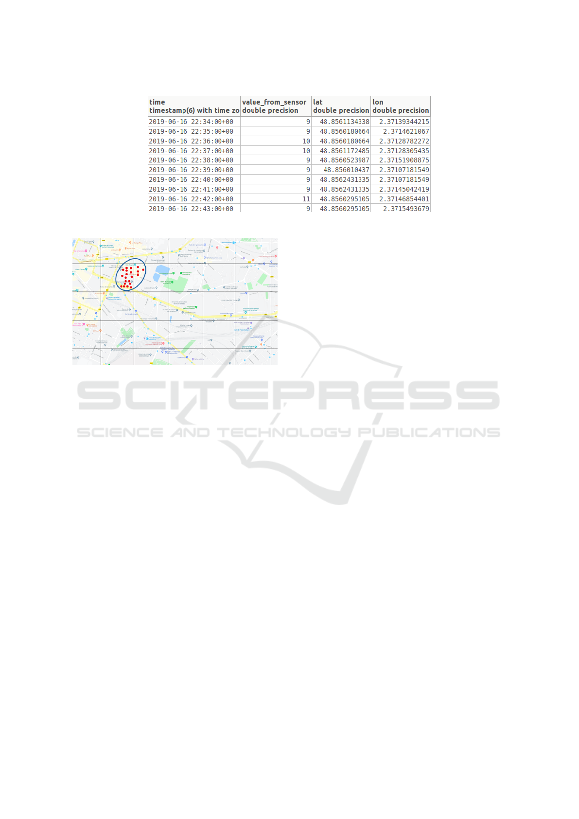
Figure 1: Snapshot of the data captured by a sensor.
Figure 2: Map showing the spread of the measurements
over the grids.
ments from all sensors carried by this participant
during their volunteering period in the campaign.
Such completeness indicator allows for better ex-
posure quantification to air pollutants for this par-
ticipant.
• Completeness for a spatial area in one campaign
is another facet which represents the spatial cov-
erage of a designated area. It indicates the spa-
tial dispersion of the measurements over this area.
The goal is to understand the way measurements
are distributed in the considered area of study, and
whether the measurements are focused in a lim-
ited part of the designated area, or if they cover
all of it.
• Temporal Completeness characterizes the way a
given period of time is covered by the collected
measurements. These measurements may have
been collected at regular intervals throughout the
period, or taken in specific chunks of time, leav-
ing other chunks without any measurement. As-
sessing such completeness assumes that the rate
at which the sensors are supposed to provide their
measurements is known.
• Sensor Completeness which is an indicator that
reflects the completeness of one specific sensor
throughout the duration of the campaign. As one
sensor could be used by different participants at
different times during one campaign, the study of
sensor completeness over a campaign shows the
extent to which this sensor has provided the ex-
pected measurements regardless of the participant
carrying this sensor.
In the following sections, we will present the defini-
tions and metrics for three of the completeness facets
presented above: sensor, spatial and temporal com-
pleteness.
4 SENSOR COMPLETENESS
Sensor completeness is a facet of completeness that
studies how complete the measurements of one sen-
sor are over a campaign. It shows the completeness
of the data captured and sent by this specific sensor
during this campaign. The nature of the sensors
can be faulty and prone to many points of failures.
Studying their completeness can show how reliable
these sensors are by giving information about the
completeness of the data captured and sent by each
one.
Within the Polluscope project, a sensor may
only be used by one participant at a time, but it can
be used multiple times throughout the duration of the
campaign. To study the completeness of one sensor
in one campaign, we ought to study its completeness
every time it was used in that specific campaign.
Hence, if a sensor has been used 4 times during a
campaign, we have to study its completeness for each
of these 4 times.
To compute the completeness of a specific sensor S
i
,
we follow the steps below:
• Lookup all the kits where sensor S
i
has been used
in the campaign.
• Evaluate sensor completeness for sensor S
i
in each
kit separately.
Completeness Issues in Mobile Crowd-sensing Environments
131
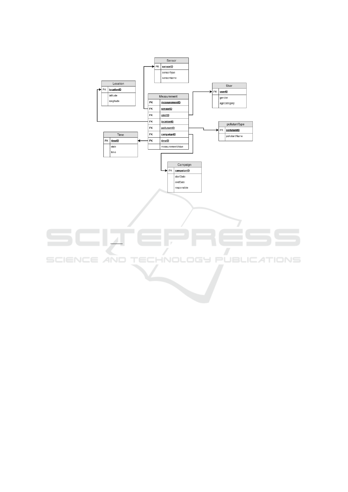
Figure 3: A Multi-Dimensional Schema for Pollution Data.
• Aggregate the computed evaluations for each kit
to calculate the completeness of sensor S
i
.
The completeness for a single sensor S
i
in one cam-
paign is evaluated as follows:
SenC
Si
=
AM
Si
RM
Si
(1)
Where AM
S
i
is the actual number of measure-
ments sensor S
i
has taken during all its usages in
one campaign. RM
S
i
is the required number of
measurements sensor S
i
must have taken during its
usages in this campaign.
The required number of measurements RM
S
i
for
a sensor S
i
throughout a campaign is defined as:
RM
S
i
= Σ
P
j=1
n
Si j
(2)
Where P is the number of kits where sensor S
i
has
been used in the campaign and n
Si j
is the number of
required measurements for sensor S
i
in kit j.
For every single usage or kit denoted j including
the sensor S
i
, n
Si j
is computed as follows:
n
Si j
= f
Si
∗ D
C j
(3)
Where f
Si
is the sampling rate of the sensor S
i
and
D
C j
is the duration of this sensor’s usage in kit j.
5 SPATIAL COMPLETENESS
Spatial completeness is the extent to which data suffi-
ciently represents a specific spatial area, and it charac-
terizes the coverage of this area considering the avail-
able measurements. In other words, spatial complete-
ness indicates how sufficient and comprehensive the
current measurements are for a particular area. This
notion is the same as the concept of data skewness
(Belussi et al., 2018).
Comprehensiveness of measurements does not neces-
sarily mean the more the better. It only means that we
have enough measurements to cover the whole area
of study and that the measurements are evenly dis-
tributed over it. This means that the measurements
taken by the sensor are not located in few portions of
the area but instead, are spread evenly all over it.
To assess spatial completeness, we may ask the fol-
lowing questions: do we have enough measurements
in this area to say that we have fully covered it?
Are the measurements evenly spread over the area of
study? Or are the measurements focused in one part
of the area being studied?
The evaluation of spatial completeness of the data
considering a designated area is performed as follows:
• Divide the area of study into equal-sized grid cells
• Compute the required number of measurements
for each grid cell and evaluate the spatial com-
pleteness for each grid cell
• Aggregate the computed evaluations for each grid
cell into the spatial completeness for the entire
area of study
Assume we want to compute the spatial completeness
of an area A. We first start by dividing the area into
equal-sized grid cells. Next, we compute the required
WEBIST 2020 - 16th International Conference on Web Information Systems and Technologies
132

number of measurements for each grid cell and the ac-
tual number of measurements taken in this grid cell.
With the actual and required number of measurements
computed, we then calculate spatial completeness for
each grid cell. Finally, the average of all cells evalu-
ations is computed to calculate the total spatial com-
pleteness for the whole area of study A.
5.1 Spatial Completeness of a Cell C
i
After dividing the designated area of study into equal
sized grid cells, we compute the spatial completeness
for each cell in the grid. Spatial completeness of a
grid cell C
i
, denoted SC
i
, is computed as follows:
SC
i
=
AM
C
i
RM
C
i
(4)
Where AM
C
i
is the actual number of measurements
in a grid cell C
i
and RM
C
i
is the required number of
measurements in a grid cell C
i
.
Different assumptions could be made in order to
estimate RM
C
i
, the required number of measurements
in a given cell. Two of them are presented hereafter:
• Hypothesis 1: The measurements are uniformly
distributed over the area of study A. In prac-
tice, this means that the number of measurements
should be evenly distributed over the cells in the
grid. Hence the required number of measurements
is:
RM
C
i
=
AM
|A|
(5)
Where AM is the actual number of available mea-
surements for the whole grid. |A| is the number of
grid cells in the area A.
• Hypothesis 2: The measurements are distributed
considering the variation of pollutant levels in the
different cells of the area of study A. Pollutant
variability could be learned from existing data ob-
tained from previous campaigns. If for a given
cell the data shows that there is a low variation of
pollutant levels in all the spatial area represented
by this cell, then the number of required measure-
ments for this cell can be low without a loss of
coverage. Conversely, if there is a high variability
in a given cell, then the required number of mea-
surements should be higher to better represent this
cell.
The value of SC
i
ranges from 0 to 1. A value
of 1 meaning that the available measurements have
an ideal distribution over the considered area. A
low value represents the fact that the measurements
are unevenly distributed over the area. Note that a
high spatial completeness value does not represent the
fact that a high number of measurements is available,
but that the available measurements, regardless of the
quantity, are more evenly distributed.
5.2 Spatial Completeness of an Area A
After computing spatial completeness for each cell in
the grid separately, the overall spatial completeness
for the whole area of study A is computed by aggre-
gating spatial completeness of all the cells. This could
be done in different ways, for example using the aver-
age, the median, the minimum or the maximum func-
tions.
We propose two quality metrics to compute the
overall spatial completeness:
• Spatial Completeness Metric 1: The first way of
evaluating spatial completeness is to compute the
average of cells spatial completeness, as shown in
the formula below:
SC(A) =
∑
|A|
i=1
SC
Ci
|A|
(6)
Where SC
Ci
is the spatial completeness of one grid
cell C
i
. |A| is the number of cells in the grid cov-
ering area A.
• Spatial Completeness Metric 2: Another way of
evaluating spatial completeness is to compute the
proportion of cells having their spatial complete-
ness above a given threshold t, as shown in the
formula below:
SC
(A)
=
∑
|A|
i=1
α
i
|A|
(7)
where
(
α
i
= 1 i f SC
Ci
≥ t
α
i
= 0 i f SC
Ci
< t
6 TEMPORAL COMPLETENESS
Temporal completeness is another facet of data com-
pleteness which can be relevant in the context of MCS
environments. It expresses the extent to which a con-
sidered period of time is well covered by the available
measurements. We consider that temporal complete-
ness states whether the measurements at hand are suf-
ficiently taken at various and comprehensive times of
the considered period or not.
We would like to characterize the extent to which
the considered period is covered in order to have an
estimate of the missing significant measurements that
could have provided an added value to the analysis
of human exposure to pollution. A high number
Completeness Issues in Mobile Crowd-sensing Environments
133

of measurements does not necessarily mean high
temporal completeness. If these measurements are
mainly taken in a small fraction of the considered
period, then the temporal completeness will be
low. However, if these measurements are evenly
distributed over the period of time, then this will
lead to a higher temporal completeness. On one
hand, sensors capturing measurements with a high
frequency, for example every minute, may at some
point add redundancy to the data, but on the other
hand, a low frequency will bring us to the problem of
missing data. It would be very useful to have addi-
tional knowledge about the distribution and variation
of the pollutants over time. For instance, in big cities,
during rush hours (5pm to 7pm) the pollutant levels
will be high and after that they diminish. However,
at the same place after midnight, it is less likely that
we observe either high variations or high levels of
pollutants.
The evaluation of temporal completeness for a
specified period of study is done as follows:
• First, divide the period of study P into equal-sized
chunks of time as it is shown in Figure 4
• Then compute the required number of measure-
ments and evaluate the temporal completeness for
each chunk.
• Aggregate the computed evaluations to calculate
the overall temporal completeness of period P.
To study the temporal completeness for a period P, we
first start by choosing the chunk size, i.e. the granu-
larity of the time unit we would like to consider. Then
we divide the period into equal-sized time chunks ac-
cording to the defined granularity. We compute the
required number of measurements and evaluate tem-
poral completeness for each chunk of time. Finally,
all chunk evaluations are aggregated to calculate the
overall temporal completeness for the period of study.
Figure 4: The time slot of period P divided into chunks C
i
.
6.1 Temporal Completeness of a
Specified Chunk of Time C
i
Different assumptions could be made in order to es-
timate the temporal completeness for a single time
chunk C
i
. Two of them are presented hereafter:
• Hypothesis 1: We consider that the measure-
ments are uniformly distributed over time. In
practice, this means that the number of measure-
ments is evenly distributed over the chunks of
time in the period to be studied. Hence, the tem-
poral completeness for a single time chunk C
i
is:
TC
i
=
AM
Ci
RM
Ci
(8)
Where AM
Ci
is the actual number of measure-
ments in a chunk of time C
i
and RM
Ci
is the re-
quired number of measurements in the chunk of
time C
i
.
RM
C
i
is defined for a chunk of time C
i
as:
RM
C
i
= Σ
K
j=1
n
s j
(9)
Where K is the number of sensors, n
s j
is the
number of required measurements for sensor s
j
during the time chunk C
i
.
For a sensor s
j
, the number of required measure-
ments during a chunk of time C
i
is computed as:
n
s j
= f
s j
∗ |C
i
| (10)
Where f
s j
is the sampling rate of the sensor s
j
ex-
pressed in number of measurements per minute,
and |C
i
| is the size of the chunk C
i
expressed in
minutes.
• Hypothesis 2: We consider that the measure-
ments are distributed considering the variation
of pollutant levels at different times of the day,
month or year. Pollutants measurements are
highly affected by time (e.g. rush hours pollutant
readings are higher than other times of the day). A
possible approach would be to analyze the avail-
able data to detect variation patterns. The number
of required measurements can then be set using
these patterns in order to compute the temporal
completeness.
6.2 Temporal Completeness of a Period
P
The temporal completeness of a period of time P pro-
vides information about the way the available mea-
surements are distributed over P, and how well P is
covered by these measurements. It is computed by
aggregating the temporal completeness values com-
puted for all the time chunks in P.
Temporal completeness for a time period P can be
computed as the average of all the temporal complete-
ness values of its chunks, as shown below:
TC
P
=
Σ
|P|
i=1
TC
i
|P|
(11)
WEBIST 2020 - 16th International Conference on Web Information Systems and Technologies
134

Where |P| is the number of chunks in a period of time
P, and TC
i
the temporal completeness of chunk C
i
.
7 EVALUATIONS
In this section, we present a preliminary assessment
of the concepts and metrics discussed in this paper.
Our experiments are done on the real data collected in
the context of the Polluscope project over two cam-
paigns that were organized in 2019. In this section,
we present preliminary evaluations of the spatial, tem-
poral and sensor completeness of the collected data
using the metrics defined in this paper.
7.1 Context of the Experiments
The Polluscope project is a multidisciplinary project
aiming at quantifying individual exposure to air pol-
lution in the region of
ˆ
ıle-de-france. During the
first phase of the project, studies and experiments on
pollutants and sensors were performed. The mea-
sured pollutants are: PM1.0, PM2.5, PM10 (partic-
ulate matter of diameters 1.0, 2.5 and 10 respec-
tively), NO2 and BC (black carbon). Multiple sensors
were selected to measure different pollutants, the Ca-
narin sensors are used to measure PM1.0, PM2.5 and
PM10, Cairsens sensors to measure NO2 and Ae51
sensor to measure BC. The Canarin sensor also mea-
sures meteorological data such as temperature, hu-
midity and pressure.
For data acquisition, volunteers carry kits containing
sensor units with them during their daily life routines
(indoor-outdoor) without any preset routes or destina-
tions. A kit may contain one or more than one sensor,
each measuring a different pollutant, in addition to a
tablet capturing timed geo-location data.
7.2 Setup
We conducted our experiments on a Intel(R)
Core(TM) i5-8250U CPU @ 1.60GHz machine with
16GB System Memory and clock 100MHz. The data
is stored on Postgres in a docker container on the
cloud. We have used Python on Jupyter Notebook to
establish a connection with the server containing the
data and to be able to access the data for our evalu-
ations. Sensors sampling rate is 1 measurement per
minute.
7.3 Results
We selected one sensor measuring NO2 and we eval-
uated its completeness in both campaigns 1 and 2.
In campaign 1, the sensor we studied had a total of
21 398 measurements while in campaign 2, it had 38
834 measurements. Sensor completeness was 58.66%
and 59.92% in campaign 1 and 2 respectively. Ta-
ble 1 shows the detailed sensor completeness of the
selected sensor in all kits using it during campaign 2.
Table 1: Computed Sensor Completeness of a sensor mea-
suring NO2 in kits using this sensor during campaign 2.
kit Nb Sen-Comp Start date End date
55 37.65% 2019-10-18 2019-10-27
70 77.3% 2019-10-30 2019-11-08
82 70.20% 2019-11-13 2019-11-23
92 28.55% 2019-11-29 2019-12-08
107 87.89% 2019-12-12 2019-12-20
Over the two campaigns 1 and 2 conducted from 15-
05-2019 to 15-09-2019 and from 15-10-2019 to 01-
01-2020 respectively, we evaluated spatial complete-
ness for each of the pollutants: PM1.0, PM2.5, PM10,
NO2, BC and also for measurements related to me-
teorological data such as humidity, temperature and
pressure. The evaluations are done over a manually
selected area in Paris. Our experiments were done on
a total number of measurements for the selected pol-
lutants and meteorological data in campaign 1 with 1
627 487 measurements and 4 229 053 measurements
in campaign 2.
Campaign 1 has 27 kits, we first compute spatial
completeness as explained in section 5 for a pollutant
for each of the kits, and then we compute an aver-
age of all the kits to get the total spatial complete-
ness. Campaign 2 comprises 63 kits, this should be
taken into consideration when analyzing spatial com-
pleteness as there are more kits, which means a higher
probability of a wider spatial coverage. Table 3 shows
the spatial completeness values computed for cam-
paigns 1 and 2.
Table 2: Computed Spatial Completeness of all pollutants
during each sensing campaign.
Pollutants SC Campaign 1 SC Campaign 2
PM1.0 15.10% 33.02%
PM2.5 15.10% 33.02%
PM10 15.10% 33.02%
NO
2
18.17% 35.15%
BC 20.38% 34.99%
Temperature 15.10% 32.91%
Humidity 15.10% 32.91%
Pressure 15.10% 33.024%
Over the two campaigns 1 and 2, we also evalu-
ated temporal completeness for each of the pollutants:
PM2.5, NO
2
and BC. The project’s kits use three dif-
ferent sensors to measure the 3 aforementioned pol-
Completeness Issues in Mobile Crowd-sensing Environments
135

lutants. For the temporal completeness evaluations,
we had 582 506 measurements of the 3 selected pol-
lutants in campaign 1 and 1 378 497 measurements in
campaign 2.
Campaign 1 has 27 kits while campaign 2 has 63.
Table 3 shows the total aggregated average of each
pollutant during each campaign. Temporal Complete-
ness for each kit is computed as explained in section
6 for every pollutant over each campaign’s time dura-
tion.
Table 3: Aggregated total average of Temporal Complete-
ness of all pollutants during each sensing campaign.
Pollutants TC Campaign 1 TC Campaign 2
PM2.5 7.75% 42.23%
NO
2
60.91% 63.66%
BC 68.53% 59.49%
7.4 Discussion
The Sensor Completeness evaluations were disparate
as we notice sometimes the sensor completeness for
NO
2
was very high and some other times it was rel-
atively low. During the usages of the sensor in the 2
kits 55 and 92, the sensor completeness was relatively
low whereas for the other kits, the sensor complete-
ness value scored more than 70%. One possible rea-
son could be that sensors used to measure NO
2
may
sometimes lose their data if they run out of battery.
However, in overall, the sensor completeness results
were relatively high for the selected sensor measuring
NO
2
.
As for the evaluations of Spatial Completeness,
the results of campaign 2 are generally better than
those of campaign 1. Even though the measurements
in campaign 2 are better than those of campaign 1,
the spatial completeness achieved in both campaigns
is not high and this could mean that the participants
did not change their locations a lot during their par-
ticipation periods. This can make sense if we think
of the amount of time people spend in their homes
and workplaces. The spatial completeness results are
almost in the same range for both campaigns as the
sensors measuring the different pollutants we studied
were grouped in kits and carried together; the spatial
areas they cover are therefore the same. Besides, the
rates of measurement of the sensors in the setup for
the experiments was the same for all the sensors.
For the evaluation of Temporal Completeness, the
value of temporal completeness of PM2.5 and NO
2
were better at campaign 2 than in campaign 1. How-
ever, the temporal completeness in sensor measuring
BC was slightly better in campaign 1 than in 2. One
possible reason why the temporal completeness for
the sensor measuring PM2.5 is very low in campaign
1 could be that during campaign 1, the sensors were
unstable which caused the loss of many chunks of
data. Therefore, the values of campaign 2 are more
reliable for that sensor.
8 RELATED WORKS
Many research works have addressed the issues re-
lated to data quality. Some of them have studied qual-
ity dimensions and their evaluation metrics, and ex-
plained the aspects that each dimension describes and
what that tells about the data (Batini and Scannapieco,
2016), (Sidi et al., 2012), (Liu et al., 2019), (Nemani
and Konda, 2009). Some research works have also
dealt with the evaluation and assessment of data qual-
ity. In the work of (
¨
Ostman, 1997), the author de-
fined metrics and evaluated the defined quality dimen-
sions. Integrity assessment of maritime messages has
been evaluated in (Ray, 2018) through both message-
based and signal-based analysis. To help make the
decision on whether or not, allocate a sensing task,
(Wang et al., 2016) assessed the data quality of the
inferred unsensed cells in a crowdsensing environ-
ment using re-sampling methods like leave-one-out
and Bootstrap.
A data quality assessment framework has been
proposed in the work of (de Aquino et al., 2019).
(Dasu et al., 2016) proposed two types of data qual-
ity checks, the first monitors data gathering process
and checks how the arriving data looks while the sec-
ond monitors quality of the content and studies data
quality versus four defined types of constraints on the
data. The work of (Rahman et al., 2014) proposes a
supervised classification approach to assess the qual-
ity of sensor data. Using graph convolutional net-
works, (Seo et al., 2018) defines local variation and
a data quality level.
Although there are many proposals for evaluating
data quality, these proposals do not take into account
the specifics of the data in MCS environments. In our
work, we specifically assessed one quality dimension,
data completeness, with its different understandings,
as one of the main issues introduced by mobile sen-
sors is the loss of data.
Some works have also addressed quality evalua-
tion at the sensor level such as (Fishbain et al., 2017)
who proposed a toolkit for the evaluation of micro-
sensing units explaining all the factors and their met-
rics. (Languille et al., 2020) used the SET tool pro-
posed by (Fishbain et al., 2017) to evaluate the perfor-
mance of air quality sensors, and to justify selection
of certain sensors rather than the others.
WEBIST 2020 - 16th International Conference on Web Information Systems and Technologies
136

Another set of works are more focused on repre-
senting and characterizing data quality in data stor-
age systems and extending traditional existing tools
to allow the association of quality indicators to data.
(Han et al., 2010) identified two different types of
sensor applications and their respective requirements,
and proposed strategies for both the satisfaction and
the optimization of either a single requirement or
multi-dimensional quality requirements. (Mustapha
et al., 2018) proposed a multivariate spatial time se-
ries representation model and used functional data
representation for storing, aggregating, transforming
and retrieving sensor data. (Klein et al., 2007) pre-
sented a metadata model extension for a relational
database schema to store quality information along
with data values, and have also extended conventional
data stream systems to propagate data quality indica-
tors.
However, given the polysemous nature of the con-
cept of data quality, some authors try to define the
meaning of this concept according to the specific field
and context. (Han et al., 2010) characterized two
types of data requirements under which they catego-
rized each quality dimension. (Rodr
´
ıguez and Servi-
gne, 2013) defined the quality dimensions for envi-
ronmental monitoring systems and (
¨
Ostman, 1997)
defined the quality dimensions for spatial data. In ad-
dition, (Ferreira and Ferreira, 2017) defined and il-
lustrated the data dimensions that are useful for the
context of Mobile Sensing. While these works aim
at discussing the application of all data dimensions to
mobile sensing environments, we focus in our work
on one of these dimensions, namely data complete-
ness, we characterize it, we study its different facets
and we propose some suitable evaluation metrics. Ac-
curacy and completeness are the most commonly de-
scribed and evaluated dimensions for mobile sensing
in the existing works. One of these works addressed
specifically completeness assessment (Biswas et al.,
2006), and the authors developed a quality model to
assess data completeness for sensor data by translat-
ing data rates to completeness values measured over
a period of time. They considered a specific ”smart
home” application context to demonstrate how com-
pleteness can be calculated. Similarly to this work,
we also use the sampling/data rate to evaluate com-
pleteness, but we also introduce and discuss the dif-
ferent facets of completeness for the context of mo-
bile crowd-sensing and assess completeness spatially,
temporally and for a specific sensor.
9 CONCLUSION
This paper is a first attempt towards characterizing
and monitoring data quality in mobile crowd-sensing
environments. We have first introduced a multi-
dimensional data model to represent sensor data in
this context. Then we have focused on data com-
pleteness and presented its different facets. We have
provided the definitions and the evaluation metrics
for three of these facets: sensor completeness, spatial
completeness and temporal completeness. We have
performed some evaluations of the proposed met-
rics on real mobile sensor data from the Polluscope
project, aiming at measuring and analysing air qual-
ity. The results on the different facets of completeness
show that it is useful to study this quality dimension
from different and complementary perspectives.
Beyond data completeness evaluation, our future
works will address the improvement of data com-
pleteness, and we will tackle the problem of generat-
ing missing values in mobile crowd-sensing environ-
ments, taking into account the available knowledge
about the quality of the sensors as well as the recorded
activities of the participants carrying them. We will
also study other quality problems such as detecting
and correcting the anomalies in the collected data.
ACKNOWLEDGEMENTS
This work is supported by the Polluscope project
(grant ANR-15-CE22-0018 of the French National
Research Agency) and the Qualiscope Impulsion
project (I-SITE FUTURE, Gustave Eiffel University).
REFERENCES
Batini, C. and Scannapieco, M. (2016). Data and Informa-
tion Quality - Dimensions, Principles and Techniques.
Data-Centric Systems and Applications. Springer.
Belussi, A., Migliorini, S., and Eldawy, A. (2018). De-
tecting skewness of big spatial data in SpatialHadoop.
GIS: Proceedings of the ACM International Sympo-
sium on Advances in Geographic Information Sys-
tems, pages 432–435.
Biswas, J., Naumann, F., and Qiu, Q. (2006). Assessing
the completeness of sensor data. In Lee, M., Tan, K.,
and Wuwongse, V., editors, Database Systems for Ad-
vanced Applications, 11th International Conference,
DASFAA 2006, Singapore, April 12-15, 2006, Pro-
ceedings, volume 3882 of Lecture Notes in Computer
Science, pages 717–732. Springer.
Dasu, T., Duan, R., and Srivastava, D. (2016). Data Quality
for Temporal Streams. Technical report.
Completeness Issues in Mobile Crowd-sensing Environments
137

de Aquino, G. R. C., de Farias, C. M., and Pirmez, L.
(2019). Hygieia: data quality assessment for smart
sensor network. In Hung, C. and Papadopoulos, G. A.,
editors, Proceedings of the 34th ACM/SIGAPP Sym-
posium on Applied Computing, SAC 2019, Limassol,
Cyprus, April 8-12, 2019, pages 889–891. ACM.
Ferreira, E. and Ferreira, D. (2017). Towards altruis-
tic data quality assessment for mobile sensing. In
Lee, S. C., Takayama, L., and Truong, K. N., ed-
itors, Adjunct Proceedings of the 2017 ACM Inter-
national Joint Conference on Pervasive and Ubiqui-
tous Computing and Proceedings of the 2017 ACM In-
ternational Symposium on Wearable Computers, Ubi-
Comp/ISWC 2017, Maui, HI, USA, September 11-15,
2017, pages 464–469. ACM.
Fishbain, B., Lerner, U., Castell, N., Cole-Hunter, T.,
Popoola, O., Broday, D., I
˜
niguez, T., Nieuwenhuijsen,
M., Jova
ˇ
sevi
´
c-Stojanovi
´
c, M., Topalovic, D., Jones,
R., Galea, K., Etzion, Y., Kizel, F., Golumbic, Y.,
Baram Tsabari, A., Yacobi, T., Drahler, D., Robinson,
J., and Bartonova, A. (2017). An evaluation tool kit of
air quality micro-sensing units.
Han, Q., Hakkarinen, D., Boonma, P., and Suzuki, J. (2010).
Quality-aware sensor data collection. International
Journal of Sensor Networks, 7(3):127.
Klein, A., Do, H. H., Hackenbroich, G., Karnstedt, M.,
and Lehner, W. (2007). Representing data quality for
streaming and static data. Proceedings - International
Conference on Data Engineering, (January 2014):3–
10.
Languille, B., Gros, V., Bonnaire, N., Pommier, C.,
Honor
´
e, C., Debert, C., Gauvin, L., Srairi, S., Annesi-
Maesano, I., Chaix, B., and Zeitouni, K. (2020). A
methodology for the characterization of portable sen-
sors for air quality measure with the goal of deploy-
ment in citizen science. Science of The Total Environ-
ment, 708:134698.
Liu, C., Nitschke, P., Williams, S., and Zowghi, D. (2019).
Data quality and the internet of things. Computing.
Mustapha, A., Zeitouni, K., and Taher, Y. (2018). To-
wards rich sensor data representation - functional data
analysis framework for opportunistic mobile monitor-
ing. In Grueau, C., Laurini, R., and Ragia, L., edi-
tors, Proceedings of the 4th International Conference
on Geographical Information Systems Theory, Appli-
cations and Management, GISTAM 2018, Funchal,
Madeira, Portugal, March 17-19, 2018, pages 290–
295. SciTePress.
Nemani, R. R. and Konda, R. (2009). A framework for
data quality in data warehousing. In Yang, J., Ginige,
A., Mayr, H. C., and Kutsche, R., editors, Information
Systems: Modeling, Development, and Integration,
Third International United Information Systems Con-
ference, UNISCON 2009, Sydney, Australia, April 21-
24, 2009. Proceedings, volume 20 of Lecture Notes
in Business Information Processing, pages 292–297.
Springer.
¨
Ostman, A. (1997). The specification and evaluation of spa-
tial data quality. Proceedings of the 18st International
Cartographic Conference, pages 836–847.
Rahman, A., Smith, D. V., and Timms, G. (2014). A novel
machine learning approach toward quality assessment
of sensor data. IEEE Sensors Journal, 14(4):1035–
1047.
Ray, C. (2018). Data variety and integrity assessment for
maritime anomaly detection. CEUR Workshop Pro-
ceedings, 2343:4–7.
Rodr
´
ıguez, C. C. G. and Servigne, S. (2013). Managing
Sensor Data Uncertainty. International Journal of
Agricultural and Environmental Information Systems,
4(1):35–54.
Seo, S., Mohegh, A., Ban-Weiss, G., and Liu, Y. (2018).
Automatically inferring data quality for spatiotempo-
ral forecasting. In International Conference on Learn-
ing Representations.
Sidi, F., Panah, P. H. S., Affendey, L. S., Jabar, M. A.,
Ibrahim, H., and Mustapha, A. (2012). Data qual-
ity: A survey of data quality dimensions. In Mah-
mod, R., Abdullah, R., Abdullah, L. N., Sembok, T.
M. T., Smeaton, A. F., Crestani, F., Doraisamy, S.,
Kadir, R. A., and Ismail, M., editors, 2012 Interna-
tional Conference on Information Retrieval & Knowl-
edge Management, Kuala Lumpur, Malaysia, March
13-15, 2012, pages 300–304. IEEE.
Wang, L., Zhang, D., Wang, Y., Chen, C., Han, X., and
M’Hamed, A. (2016). Sparse mobile crowdsensing:
Challenges and opportunities. IEEE Communications
Magazine, 54(7):161–167.
WEBIST 2020 - 16th International Conference on Web Information Systems and Technologies
138
