Batch Contrastive Regularization for Deep Neural Network

Muhammad Tanveer

, Hung Khoon Tan

, Hui Fuang Ng

Maylor Karhang Leung

and Joon Huang Chuah

Faculty of Information and Communication Technology, Universiti Tunku Abdul Rahman, Malaysia

Faculty of Engineering, Universiti Malaya, Malaysia

Keywords: Batch Contrastive Loss, Batch Regularization, Center-level Contrastive Loss, Sample-level Contrastive Loss,

Neural Network.

Abstract: As neural network becomes deeper, it becomes more capable of generating more powerful representation for

a wide variety of tasks. However, deep neural network has a large number of parameters and easy to overfit

the training samples. In this paper, we present a new regularization technique, called batch contrastive

regularization. Regularization is performed by comparing samples collectively via contrastive loss which

encourages intra-class compactness and inter-class separability in an embedded Euclidean space. To facilitate

learning of embedding features for contrastive loss, a two-headed neural network architecture is used to

decouple regularization classification. During inference, the regularization head is discarded and the network

operates like any conventional classification network. We also introduce bag sampling to ensure sufficient

positive samples for the classes in each batch. The performance of the proposed architecture is evaluated on

CIFAR-10 and CIFAR-100 databases. Our experiments show that features regularized by contrastive loss has

strong generalization performance, yielding over 8% improvement on ResNet50 for CIFAR-100 when trained

from scratch.

1 INTRODUCTION

As neural networks (He et al., 2016; Zagoruyko et al.,

2016; Xie et al., 2017) become deeper over the years,

it has become more adept at tackling more complex

classification and detection tasks. However, deeper

networks have a large number of parameters which

makes it more prone to overfitting especially when

trained on a small training set. Different

regularization methods have been designed over the

recent years to improve generalization performance.

Widely used techniques include weight decay (Krogh

et al., 1992), data augmentation (Shorten et al., 2019),

and dropout (Srivastava et al., 2014). In general, these

techniques inject random noise into the network

(Srivastava et al., 2014) or data samples (Shorten et

al., 2019) when training the network. One common

feature of these techniques is that samples are treated

individually. Although training is carried out in

https://orcid.org/0000-0001-9964-7186

https://orcid.org/0000-0003-4394-2770

https://orcid.org/0000-0002-1023-7162

https://orcid.org/0000-0001-9058-3497

batches, most computations (e.g., forward

propagation, loss, regularization and propagation) are

done with little interaction between the samples

except for simple averaging at the end.

Recently, batch loss regularization techniques

(Wen et al., 2016; Huang et al., 2017; Zhao et al.,

2019) explores how to regularize a network

collectively by tapping into the relationship between

batch samples. Compared to the softmax loss (Figure

1(a)) which learns separable decision boundaries,

center loss (Wen et al., 2016) further encourages

intra-class compactness (Figure 1(b)) by penalizing

the distance between embedding features and their

corresponding centers. Exclusive regularization

(Zhao et al., 2019) additionally ensures that the

centers are far apart by penalizing the angles between

two neighbouring centers (Figure 1(c)). The

generated features are more representative and

discriminative.

368

Tanveer, M., Tan, H., Ng, H., Leung, M. and Chuah, J.

Batch Contrastive Regularization for Deep Neural Network.

DOI: 10.5220/0010135303680377

In Proceedings of the 12th International Joint Conference on Computational Intelligence (IJCCI 2020), pages 368-377

ISBN: 978-989-758-475-6

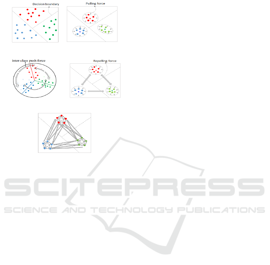
Figure 1: Embedding features trained under various loss

functions. (a) Softmax loss generates embedding features

that are separable (b) Center loss (Wen et al., 2016) ensures

intra-class compactness. (c) Exclusive regulation (Zhao et

al., 2019) ensures both intra-class compactness and inter-

class separability using angular loss (d) Our proposed

center contrastive loss uses the contrastive loss function in

an euclidean embedding space. (e) Our proposed sample

contrastive loss is similar to (d) except that the distance is

computed between sample-pairs.

Intra-class compactness and center separability

apparently exhibit promising regularizing effect.

Interestingly, some studies in perceptual learning

(Mitchell et al., 2014; Mundy et al. 2007) show that

the performance of human on categorization task can

be enhanced when the stimuli are presented side by

side so that the subject is given the opportunity for

comparison. In (Mundy et al., 2007), human subjects

were found to perform better at categorization tasks

when two stimuli such as face pairs or checkerboard

pattern pairs were presented simultaneously as

opposed to successively. Interestingly, the ability to

learn from comparison is potentially unique to

human, not found in animal, which shows that

learning from simultaneous samples represents a

higher order of learning.

In this paper, we novelly use contrastive loss to

realize batch loss regularization. Contrastive loss has

been widely adopted for distance metric learning.

More importantly, features generated from

contrastive loss has been shown to deliver superior

performance for a multitude of tasks compared to

softmax loss when the training set is small (Horiguchi

et al., 2019). Hence, we posit that the network

regularized by contrastive loss has good

generalization property. We explore two different

contrastive losses: (1) the center contrastive loss

shown in Figure 1(d) which uses embedding feature

centers as the reference point and (2) the sample

contrastive loss shown in Figure 1(e) which is based

on sample-pair distances.

Our contribution are as follows. First, we propose

a novel batch loss regularization method called batch

contrastive loss. We devise two variants of batch

contrastive loss to regularize the network. Second,

our work is the first to seriously explore batch loss

regularization for general classification. Previous

works on batch loss regularization are limited to

specific domain e.g., face recognition (Wen et al.,

2016; Zhao et al., 2019), or scene classification

(Huang et al., 2017). In our experiments, our

proposed method displays strong generalization

performance for the CIFAR-100 dataset. Third, we

use a two-headed network architecture in order to

decouple regularization from classification. During

inference, the regularization head is dropped and only

the classification head remains. Lastly, we introduce

bag sampling to guarantee that the classes in a batch

are not under-represented.

2 RELATED WORK

As neural network becomes deeper, the huge number

of parameters causes the network to become prone to

overfitting especially when trained on a small

targeted dataset, leading to poor generalization

performance. To solve this problem, a number of

powerful regularization techniques have been

developed to overcome the problem. Classical

methods include weight decay (Krogh et al., 1992),

elastic net (Zou et al., 2005) and early stopping

(Morgan et al., 1990). For modern neural networks,

dropout (Srivastava et al., 2014; Wan et al., 2013;

Tompson et al., 2015; DeVries et al., 2017; Ghiasi et

al., 2018) and data augmentation (Krizhevsky et al.,

2012; Zhong et al., 2020 ; Cubuk et al., 2019) have

gained wide adoption.

Dropout (Srivastava et al., 2014) stochastically

deactivates activations in the network during training.

This causes the model to be simpler and discourages

co-adaptation among feature detectors. Drop connect

(Wan et al., 2013) further generalizes dropout by

masking connections between neurons. Standard

dropout techniques (Srivastava et al., 2014; Wan et

(a) Softmax loss (b) Center Loss (Wen

et al., 2016)

et al., 2019)

(e) Sample Contrastive Loss

Batch Contrastive Regularization for Deep Neural Network

369

al., 2013) are effective for fully connected layers but

not suited for convolutional layers which exhibits

strong spatial correlation. Hence, spatial dropout

(Tompson et al., 2015) drops an entire channel from

the feature map while cutout (DeVries et al., 2017)

and drop block (Ghiasi et al., 2018) mask out local

and contiguous regions in the input layer and

convolutional layer, respectively. Some dropout

techniques are customized for particular architecture.

For example, drop path (Larsson et al., 2016) drops

sub-paths to prevent co-adaptation of parallel paths in

a fractal architecture while stochastic depth (Huang et

al., 2016) makes a residual network appear shallower

by dropping some residual branches. Shake-shake

(Gastaldi et al., 2017) uses a stochastic affine

combination of parallel residual paths for ResNeXt

(Xie et al., 2017). To generalize shake-shake

regularization to single residual path architectures

(He et al., 2016; Zagoruyko et al., 2016; Han et al.,

2017). ShakeDrop (Yamada et al., 2018) integrates

shake-shake (Gastaldi et al., 2017) with stochastic

depth (Huang et al., 2016) where the latter acts as a

stabilization mechanism which is missing in single

residual path networks. Recent dropout techniques

has devised selective dropping schemes. For

example, spectral dropout (Khan et al., 2019) drops

less significant spectral component. Similar to spatial

dropout, weighted channel dropout (Hou et al., 2019)

drops a whole channel in a more judicious manner

based on their strength of the activations.

Another popular regularization technique is data

augmentation (Shorten et al., 2019) where a variety

of geometric and photometric transformations are

applied on the image to increase the size and diversity

of the data set. Krizhevsky et al., (2012) apply

random cropping, horizontal reflection as well as

color jittering. Algorithms such as cutout (DeVries et

al., 2017) and random erasing (Zhong et al., 2020)

augments the data by cutting out random regions from

the input image. Sample pairing (Inoue et al., 2018)

synthesize new image by mixing two images.

Recently, more intelligent augmentation schemes

have been proposed. AutoAugment (Cubuk et al.,

2019) and Fast AutoAugment (Lim et al., 2019) learn

to augment by searching for data augmentation

policies while DevVries et al. (2017) performs

transformation in a learned feature space rather than

the input space.

Our proposed method belongs to an emerging

family of regularization techniques called batch loss

regularization which regularizes batch samples

collectively. In the work by Wen et al. (2016), class

centers are computed from the embedding features of

the batch sample. Then, the center loss penalizes the

Euclidean distance between batch samples and their

corresponding centers to emphasize intra-class

compactness. The model is jointly trained by center

loss and the softmax loss. Huang et al. (2017)

employs a similar formulation for aerial scene

classification. Zhao et al. (2019) proposes exclusive

regularization which further penalizes inter-class

angular distance to enhance inter-class separability.

In our current work, we explore using a different loss

function based on batch contrastive loss to achieve

both intra-class compactness and inter-class

separability.

3 BATCH CONTRASTIVE LOSS

In this section, we formulate our proposed batch

contrastive loss. The underlying idea is to regularize

the network by comparing batch data. Given a batch

data 𝑋



𝑥



,…,𝑥





and its corresponding

labels 𝑌



𝑦



,…,𝑦





, we use a ConvNet (c.f.

Section 3) to extract two outputs: (1) the embedding

features generated by the regularization head,

henceforth referred to as contrastive features 𝐸



𝑒



,…,𝑒





and (2) the probit outputs for each sample

𝑆



𝑠



,…,𝑠





by the classification head. The former

is used to regularize the network while the latter is the

classification output of the network. The

regularization head is only used during training and is

discarded during inference. In the following sub-

sections, we introduce two versions of batch

contrastive loss functions. The first regularizes batch

samples with reference to the class centers whereas

the second regularizes based on sample-pair

distances.

3.1 Center Contrastive Loss

Our first contrastive regularization term learns the

features and class centers that enforce intra-class

compactness and inter-class separability. Distances

are measured with respect to the class centers as

reference points. The loss function is given as

follows:

ℒ





𝐸,𝑌,𝐶



𝜆𝑒



𝑐













 𝛽   max



0,𝑚  𝑐



𝑐

















(1)

where the class centers 𝐶



𝑐



,…,𝑐





are updated in

each iteration based on the mean of the batch samples

for each class.

𝑐

𝑦

𝑖

is the actual class center for the

contrastive feature 𝑒

𝑖

. The loss function is based on

the classical contrastive loss function (Chopra et al.,

2005) which comprises two parts. The first part is the

positive loss which penalizes the distance between

NCTA 2020 - 12th International Conference on Neural Computation Theory and Applications

370

generated contrastive feature with their class centers.

This encourages intra-class compactness and is

similar in form to the center loss (Wen et al., 2016).

The second part is the negative loss which pushes

class centers apart by penalizing any two centers with

distance less than the margin m. This promotes inter-

class separability. The relative strength of the positive

and negative losses can be controlled by the

hyperparameters 𝜆 and 𝛽. A larger 𝜆 enhances the

intra-class compactness whereas a larger 𝛽 imposes

greater inter-class separability.

Since the distances are computed relative to the

class centers, we refer to Eq. (1) as the center

contrastive loss. The proposed center-level

contrastive regularization term is similar in form to

Zhao et al. (2019). However, Zhao et al. (2019) uses

an angular distance measure which disregards the

magnitude of the embedding vectors. In contrast, our

method employs the contrastive loss formulation

(Chopra et al., 2005) which is based on straight-line

distance in an Euclidean space. Contrastive loss has

been popularly used for the task of metric learning but

has never been used for batch loss regularization.

Furthermore, Horiguchi et al. (2019) shows that it is

more effective to use angular distance when

comparing embedding features extracted from a

softmax-based classifier. Since Zhao et al. (2019)

employs the same features for computing softmax

(classification) loss and exclusive (regularization)

loss, it has naturally adopted the angular-based

distance. Our network does not suffer from the same

restriction due to a two-headed network design which

decouples regularization from classification. In fact,

Horiguchi et al. (2019) shows that the Euclidean

distance is more effective for comparing features

extracted from a distance metric-learning based

learning classifier as implemented by the

regularization head in our approach. More discussion

on the network architecture can be found in Section

3.3.

3.2 Sample Contrastive Loss

The cluster contrastive regularization proposed in the

previous section is efficient, but it restricts each class

to a single class center which may not be desirable for

classes with high-intra-class variation. Furthermore,

the cluster centers are dynamically updated in each

iteration based on batch data and may not be

representative of the whole dataset. Hence, we

propose a second loss function which performs

regularization at the sample level. It is based on the

vanilla contrastive loss function. Recently, one-shot

learning (Koch et al., 2015) uses Siamese network to

learn using a single example of a new class. The

network was pre-trained for some verification task

using contrastive loss by comparing image pairs.

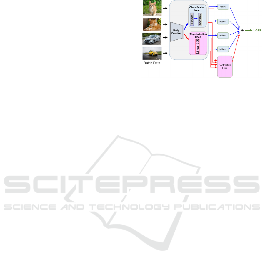
Figure 2: Proposed two-headed network architecture. The

body of the network generates the activation map. The

regularization head is used. The classification head is a

softmax classifier. For inference, the regularization head is

dropped.

Once optimized, the network is not only

discriminative for the original classes it was trained

on, but it generalizes well to learn entirely new

classes with unknown distribution. Motivated by this

observation, we adopt the contrastive loss as a

regularization term to tap into the generalization

capability of contrastive features. The sample

contrastive loss is given as follows:

ℒ





𝐸,𝑌



 𝜆𝟏𝑦



𝑦



𝑒



𝑒















𝛽𝟏𝑦



𝑦



max



0,𝑚  𝑒



𝑒











(2)

𝟏



∙



is an indicator function that values to 1 when the

condition is true

and to 0 otherwise.

The first term

computes the distance for all positive pairs in the

batch. The second term computes the negative loss

which penalizes when the distance between any two

negative samples are less than m. Since the distances

are measured sample-wise, we refer to Eq. 2 as

sample contrastive loss.

Our work differs from the work Koch et al. (2015)

in two important aspects. The system by Koch et al.,

(2015) is designed to function as a comparator.

Hence, the constructed model is a bi-input model that

expects two input samples even during inference and

outputs the distance between them. In contrast, (i) we

use contrastive loss for a different purpose, i.e., to

regularize the training and (ii) our network remains as

a uni-input model and receives single sample as input

during inference. Hence, our method can be applied

to any classification tasks and not confined to a

comparative setup.

Compared to center contrastive loss (Eq. 1), the

sample contrastive loss (Eq. 2) incurs some

computational overhead due to an exhaustive

computation of pair-wise distances between sample

Batch Contrastive Regularization for Deep Neural Network

371

pairs in a batch, especially when a large batch size is

used. The time complexity involved is O(N

). In our

experiments, the training duration increases to 1.5

times of the original training time for a batch size of

16. However, this can be easily overcome by

combining hashing and hard sampling (Hermans et

al., 2017). An off-the-shelve nearest neighbour

search, e.g., LSH (Indyk et al., 1998) can be used to

find the hardest positive and hardest negative to

compute the loss for each sample. The hardest

positive and negative samples are then used to

compute the triplet loss. Hard sampling has been

shown to produce better performance and

convergence rate. The runtime can thus be reduced to

O(N). In our experiments, we simply compute the

distance for all sample pairs.

3.3 Model Architecture

Figure 2 shows an overview of our network

architecture. The proposed network is a two-headed

network. The body of the network can be

implemented by any current ConvNet architecture. Its

function is to generate the features for the two heads.

The regularization head converts the feature into a

low-dimensional contrastive features (256-D) for

regularizing the network via contrastive loss whereas

the classification head is a softmax classifier to

predict the label. The classification head uses softmax

activation. No activation is imposed for the

regularization head.

Although Zhao et al. (2019) has similar design as

ours, it uses the softmax-based feature (features

extracted from a softmax classifier) to compute the

angular loss. As mentioned, softmax-based features

are more appropriately evaluated using angular

distance. In contrast, our two-headed network design

allows us to use the softmax-based feature for

classification and contrastive-based feature (feature

learnt from distance metric learning) for

regularization. A previous study (Horiguchi et al.,

2019) has pit softmax-based feature against

contrastive-based feature. It shows that the softmax-

based features perform better on classification,

clustering and retrieval tasks when the size of the

training set is large, but the contrastive-based feature

becomes more competitive when the dataset is small.

This lend strong support for using contrastive loss to

regularize the network. For inference, the

regularization head is dropped leaving only the

classification head. Hence, our network remains as a

uni-input model and works just like any other

classification model during inference.

3.4 Bag Sampling

Special attention needs to be paid to sample selection.

When sampling batch data, each class in a batch

should be represented by at least 2 samples for

contrastive regularization to be effective. However,

this requirement will likely be violated when number

of classes is larger than the batch size. For example,

ImageNet has 1000 class whereas the typical bag size

is from 4 to 256. To remedy the issue, we perform bag

sampling. In this scheme, samples are organized into

groups of k samples called bags. When sampling

batch data for training, we sample in bags rather than

individual samples. The samples in the bags are non-

overlapping except for the last one to ensure

consistent batch size. Thus, one epoch in bag

sampling performs almost the same number of

forward propagations as one epoch in conventional

sampling.

3.5 Proposed Algorithm

To measure classification performance, we use the

cross entropy loss:

ℒ





𝑆,𝑌





𝑁

log𝑠









(3)

where

𝑠





is the probit of the correct class for

sample𝑥



. To train the network, we perform joint

supervision of cross entropy loss and batch

contrastive loss. The final loss is given as follows:

ℒ



ℒ





ℒ



(4)

where the contrastive loss

ℒ



can be either ℒ





or ℒ





. The training algorithm is summarized in

Algorithm 1.

Algorithm 1: Training algorithm with Batch

Contrastive Regularization.

Input: Training data



𝑋, 𝑌



Output: Trained network weights 𝑊

1. Repeat for n epochs

2. Organize samples into bags

3. Repeat for each batch data 𝑋



(bag

sampling):

4. 𝐸,𝑆  model(𝑋



)

5. Compute cluster centers 𝐶 from 𝐸

6. Compute contrastive loss ℒ





𝐸,𝑌,𝐶



(Eq.1) or ℒ





𝐸,𝑌



(Eq. 2)

7. Compute classification loss ℒ





𝑆,𝑌



(Eq. 3)

8. Compute combined loss ℒ (Eq. 4)

9. Backpropagate and update 𝑊

NCTA 2020 - 12th International Conference on Neural Computation Theory and Applications

372

4 IMPLEMENTATION DETAILS

Network Architecture. ResNet (He et al., 2016) is

employed as the backbone of our two-headed

network. We use two networks with different depth,

namely ResNet18 and ResNet50. The output of

global pooling layer serves as input to the

regularization and classification heads. Both the

regularization head and classification has only one

fully connected layer. The classification head uses

softmax activation whereas the regularization has no

activation.

Experimental Settings. All images are resized to

224x224. For data augmentation, we apply random

crop, random horizontal flip and color jittering during

training. We set the learning rate lr=0.1, =10

-4

and

the margin m=1.25. For , we set it to 0.550 for

CIFAR-10 and 5.0 for CIFAR-100. The network is

trained for 100 epochs using stochastic gradient

descent with momentum set to 0.9. A learning rate

schedule is used with decay = 0.1 and milestone =

[50, 75]. Unless specified otherwise, for our methods,

we use bag sampling with a bag size of 2 to sample

the training set. All models are trained from scratch.

In other words, we do not use any pre-training. The

above settings are used to train both the ResNet18 and

ResNet50 backbone network.

Benchmark Algorithms. We compare our

algorithms against the weight decay (Krogh et al.,

1992) which suppresses the parameters of the

network

𝑊 through the L2 norm thus enforcing a

simpler network.

ℒ

𝛾

‖

𝑤

𝑖

‖





∈

(5)

The weight decay can also be combined with

contrastive loss.

ℒ



ℒ





ℒ



 ℒ

(6)

We also compare our algorithm with another more

recent regularization function. The center loss (Wen

et al., 2016) is similar to our center contrastive loss

(Eq 1) except that it only considers intra-class

compactness.

Center Loss



𝐸,𝑌,𝐶



𝑒



𝑐













(7)

Dataset. We evaluated on two datasets: CIFAR-

10 and CIFAR-100. CIFAR-10 has 10 distinct classes

whereas CIFAR-100 has 100 classes. Each image

contains only single object and has a size of 32  32

pixels. Both datasets contain 50,000 training images

and 10,000 test images. CIFAR-10 has around 5,000

images per class for training whereas CIFAR-100 has

only 500 images. In addition, some classes in CIFAR-

100 (e.g., maple, oak, palm, pine and willow) are

visually similar and hence difficult to classify.

Therefore, CIFAR-100 is a more challenging dataset

compared to CIFAR-10 and needs more fine-grained

classification.

5 EXPERIMENTS

Effectiveness of Batch Loss Regularization. First,

we evaluate the effectiveness of different batch loss

regularization techniques for regularizing networks.

We compare our method against another batch loss

regularization technique, namely center loss (Wen et

al., 2016). Table 1 shows the experimental result.

Table 1: Testing Accuracy of Batch Loss Regularization for

ResNet18 (No Pre-Training).

Method CIFAR-10 CIFAR-100

CE 92.20% 69.68%

CE + Center 93.00%

(

+0.80

)

67.12%

(

-2.56

)

CE + CL1 93.16% (+0.96) 73.78% (+4.10)

CE + CL2 93.18% (+0.98) 71.18%

(

+1.50

)

* CE: Cross entropy loss (no regularization), Center: Center Loss

(Wen et al., 2016), CL1: Center contrastive loss (proposed), CL2:

Sample contrastive loss (proposed).

* The numbers in the bracket indicates the improvement for the

various regularization methods compared to the baseline (no

regularization).

For CIFAR-10, center contrastive loss (CL1) and

sample contrastive loss (CL2) improve test accuracy

to 93.16% (+0.96) and 93.18% (+0.98), respectively

compared to the baseline test accuracy of 92.20%.

This shows that both contrastive losses successfully

regularize the network. The improvement is much

more pronounced for CIFAR-100. The sample

contrastive loss (CL2) improves the test accuracy

from 69.68% to 71.18% (+1.50). The improvement

for center contrastive loss (CL1) is bigger where the

test accuracy improves to 73.78% (+4.1). The impact

of regularization is more significant in CIFAR-100

since it has a less samples per class compared to

CIFAR-10.

The performance of center loss (Wen et al., 2016)

is noticeably not stable. Although delivering slight

improvement for CIFAR-10 (+0.80), it is somehow

surprising to see test accuracy drop from 69.86% to

67.12% (-2.56) after applying center loss

regularization for CIFAR-100. We offer several

possible explanations. First, to reduce computational

consideration, the centers are computed on batch

samples rather than the whole data set. Since a bag

Batch Contrastive Regularization for Deep Neural Network

373

size of 2 is used in the experiments, and there is a

relatively large number of classes (100 in CIFAR-

100), the cluster centers tend to fluctuate wildly from

batch to batch. As a result, center loss regularization

may have difficulty converging. A second plausible

explanation is intra-class variability where the visual

appearance of the samples for a class may be diverse

and the assumption of a single class center may not

be a good one for general classification tasks. This

also explains why center loss (Wen et al., 2016)

manage to deliver good regularization performance

for face recognition - there is only one single visual

category (face) and the within-class visual

appearance is not diverse. In contrast, general object

classification involves multiple classes and within-

class samples are more varied.

Compared to center loss, both versions of

contrastive loss improve test accuracy. This is

apparently attributed to the negative distances which

imposes inter-class separability. As mentioned,

CIFAR-100 contains a lot of visually similar classes,

e.g., maple, oak, palm, pine and willow. By imposing

inter-class separability into the loss function, the

network will be compelled to learn cluster centers are

well separated in the embedding space. This in turn

improves generalization performance.

Effect of Network Depth. Next, we evaluate the

effect of network depth towards regularization

performance. For this experiment, we use a deeper

network namely ResNet50 and repeat the

experiments in the previous section. Table 2 shows

the test accuracies obtained from the network.

Table 2: Testing Accuracy of Batch Loss Regularization for

ResNet50 (No Pre-Training).

Method

CIFAR-10 CIFAR-100

89.62% 63.50%

CE + Center 77.89%

(

-11.73

)

67.81%

(

+4.31

)

CE + CL1 86.45% (-3.17) 71.51% (+8.01)

CE + CL2 91.85% (+2.23) 71.92% (+8.42)

* CE: Cross entropy loss (no regularization), Center: Center Loss

(Wen et al., 2016), CL1: Center contrastive loss (proposed), CL2:

Sample contrastive loss (proposed).

Compared to ResNet18 (Table 1), the test

accuracy (without regularization) for ResNet50 drops

from 92.20% to 89.62% for CIFAR-10 and from

69.68% to 63.50% for CIFAR-100. This shows that

overfitting is more severe for ResNet50. As a deeper

network, ResNet50 contains around 25 million

parameters, which is more than double than that of

ResNet18 which has only around 11 million. This

makes ResNet50 more difficult to train and prone to

overfitting.

For CIFAR-10, when center loss is applied, test

performance drops sharply to 77.89%. Again, we

attribute this to an unstable batch center and

unrepresentative cluster center. For CL1, the

performance also drops but not as much. This shows

that the negative loss has offset the effect of the

positive loss. Sample contrastive loss regularization

improves test accuracy to 91.85% (+2.23). Here, we

notice that the performance of CL2 consistently

deliver better performance compared to the baseline

in all our experiments for networks of different depth

and dataset of different sizes. A decentralized method

with no notion of a class center seems to provide more

stable regularization in our case.

For CIFAR-100, all three batch regularization

techniques improves test accuracy performance

significantly. With no regularization, test accuracy is

63.50%. Both CL1 and CL2 see an improvement of

more than 8%, registering a test accuracy of 71.51%

(+8.01) and 71.92% (+8.42), respectively. This is

extremely significant performance improvement.

Again, center loss produces the least improvement. In

summary, batch contrastive loss displays good

generalization performance on a deeper network and

smaller samples.

Effect of Bag Sampling. Next, we evaluate the

effect of bag sampling. We evaluated 3 different bag

sizes: 0, 2 and 4. The experiment is conducted for

CE+CL2 on CIFAR-10. A batch size of 16 is used.

Note that when the bag size is 0, this is equivalent to

disabling bag sampling. Table 3 shows the result of

the effect of different bag size.

Table 3: Effect of Bag Size in Bag Sampling (CE+CL2).

Bag Size ResNet18 ResNet50

92.76% 90.70%

93.18% 91.85%

91.19%

89.84%

* CE: Cross entropy loss, CL2: sample contrastive loss.

Clearly, bag sampling improves regularization

performance for our method. The optimal bag size is

2. The test accuracy decreases when bag size

increases to 4 for both ResNet18 and ResNet50.

When the bag size increases, there are more positive

pairs and less negative pairs. As shown previously,

the performance of the positive loss (center loss) is

not stable and consequently a bigger bag size has a

negative impact on the performance of the system.

Detailed Analysis. In this section, we investigate

if the classes indeed benefit from the proposed batch

contrastive regularization. To do this, we compare the

performance of individual classes before and after

applying sample contrastive regularization (CL2).

Figure 3 shows the changes to the test accuracy after

applying CL2 on ResNet50 for CIFAR-100. Classes

NCTA 2020 - 12th International Conference on Neural Computation Theory and Applications

374

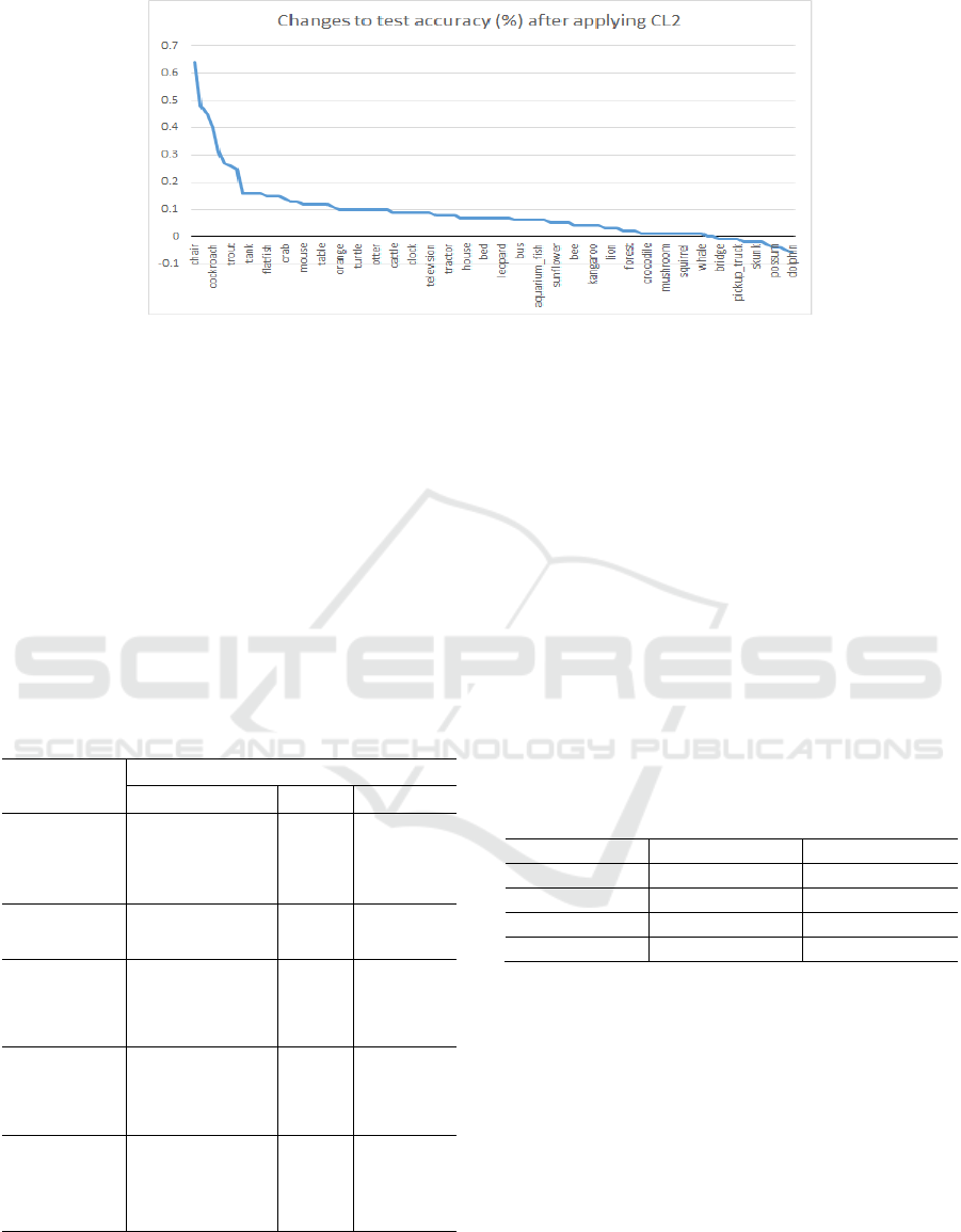
Figure 3: Changes to test accuracy for all classes after applying sample contrastive loss (CL2) of ResNet50 on the CIFAR-

100 dataset. Positive value means test accuracy improves after applying CL2 and vice versa. A huge number of classes

benefits from contrastive loss regularization. (Not all class labels are displayed in x-axis due to space constraint.

with values above the line y = 0 successfully

improve their test accuracies and vice versa. Indeed,

majority of the classes (87 out of 100) are above the

line. Out of these, 20 classes improve their accuracies

by more than 20%. This shows contrastive loss indeed

successfully regularizes the network for a wide

variety of classes.

Next, we further analyze the result for class

separability. Table 4 shows a partial confusion table

for the 5 most improved classes. Note that there are

100 test samples per class.

Table 4: Partial Confusion Table for 5 Classes without

Regularization (CE) and with Regularization (CE+CL2).

Before applying contrastive loss, these classes are

typically confused with one or two other dominant

classes. Noticeably, most are confused with hamster

and lamp most likely due to their cluttered

background. After applying the contrastive loss, the

network no longer confuses these classes.

Comparison to Weight Decay. In this section,

we compare the performance of batch contrastive loss

with weight decay (Krogh et al., 1992), or

equivalently L2 regularization. L2 is a well-trusted

technique that reduces overfitting by controlling the

network complexity by controlling the network

parameters. We repeat our experiments using L2

regularization on CIFAR10. The proposed batch loss

regularization can be additionally imposed on top of

L2. We further run our experiment with a

combination of both L2 + CL2. Table 5 shows the

result for our experiments

Table 5: Comparison with L2 Regularization on CIFAR-10

(No Pre-Training).

Metho

Res

et18 Res

et50

CE 92.20% 89.62%

CE + CL2 93.18% (+0.98) 91.85% (+2.23)

CE + L2 94.95% (+2.75) 94.54% (+5.33)

CE + L2 + CL2 95.32% (+3.12) 94.63% (+5.70)

* CE: Cross Entropy (no regularization), L2: weight decay (Krogh

et al., 1992)

, CL2: sample contrastive loss (proposed).

In the experiment, weight decay displays good

regularization performance and even outperforms

sample contrastive loss when considered separately.

When the two regularization techniques are fused

together, weight decay and the proposed contrastive

loss compensate each and deliver better

improvement. This shows that controlling the

network complexity directly by suppressing the

network parameter values still remains the most direct

and effective way of regularizing the network.

However, L2 regularization can benefit from

additionally imposing the contrastive loss.

Actual

Class

Prediction result

Predicted Class

CE CE+CL2

Chair

Chair 23 87

Hamster 45 0

Lamp 16 1

Lawn Mover

Lawn Mover 40 88

Hamster 45 0

Telephone

Telephone 27 72

Hamster 26 0

Lamp 18 4

Cockroach

Cockroach 42 92

Hamster 29 0

Beetle 5 3

Dinosaur

Dinosaur 44 75

Hamster 18 0

Lamp 9 0

Batch Contrastive Regularization for Deep Neural Network

375

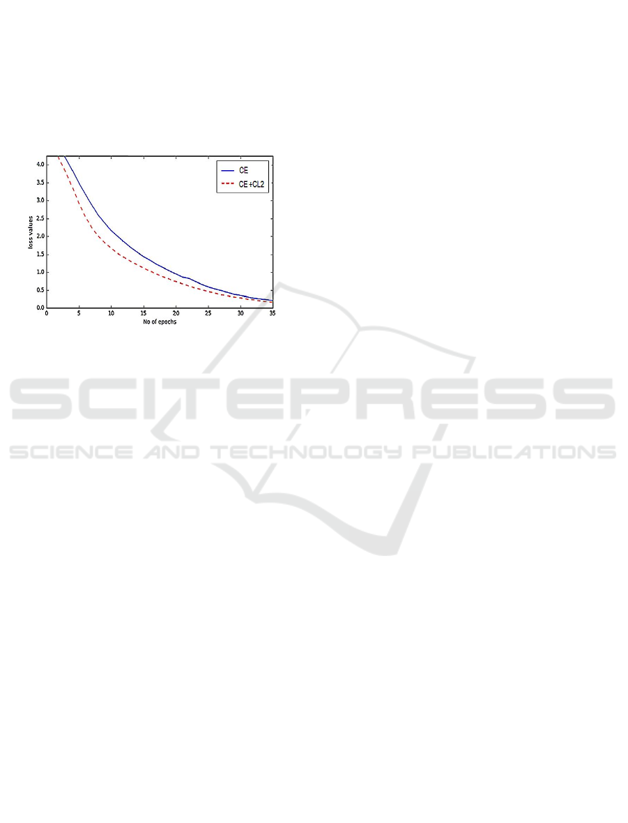
Convergence Rate. Lastly, we show the loss

function of the cross entropy (CE) loss and sample

cross entropy (CE+CL2) on ResNet50 network and

CIFAR-100 dataset to evaluate their convergence

rate. For CE + CL2, we only extract the CE

component to be plotted. Figure 4 shows the two

plots. Obviously, when the training is regulated by

sample contrastive loss, the cross entropy loss

converges faster compared to without regularization.

However, the network then converges to roughly the

same level after epoch 35. The same pattern is

observed for all other experiments.

Figure 4: The cross entropy loss for CE and CE+CL2 on

ResNet50 and CIFAR-100 dataset. For CE+CL2, only the

cross entropy loss component is used to plot the graph. With

CL2 regularization, the cross entropy converges faster.

6 CONCLUSION

Deep networks have shown impressive performance

on a number of computer vision tasks. However,

deeper networks are more susceptible to overfitting

especially when the number of samples per class are

small. In this work we introduced batch contrastive

loss to regularize the network by comparing samples

in a batch loss. Our experiments show that batch

contrastive loss has good generalization performance

especially on deeper network and dataset with smaller

number of samples per class. It also further reveals

potential issue with the positive loss for general

classification tasks which is a subject for future

investigation. In the future, we plan to perform more

evaluation to demonstrate that the technique

generalize well to other datasets as well as tasks (e.g.,

video action classification). We will also look into the

efficiency issues of contrastive loss.

ACKNOWLEDGMENT

This work was supported by a FRGS grant

(FRGS/1/2018/ICT02/UTAR/02/03) from the

Ministry of Higher Education (MOHE) of Malaysia.

REFERENCES

Chopra, S., Hadsell, R., & LeCun, Y. (2005, June).

Learning a similarity metric discriminatively, with

application to face verification. In 2005 IEEE

Computer Society Conference on Computer Vision and

Pattern Recognition (CVPR'05) (Vol. 1, pp. 539-546).

IEEE.

Cubuk, E. D., Zoph, B., Mane, D., Vasudevan, V., & Le, Q.

V. (2019). Autoaugment: Learning augmentation

strategies from data. In Proceedings of the IEEE

conference on computer vision and pattern

recognition (pp. 113-123).

DeVries, T., & Taylor, G. W. (2017). Dataset augmentation

in feature space. arXiv preprint arXiv:1702.05538.

DeVries, T., & Taylor, G. W. (2017). Improved

regularization of convolutional neural networks with

cutout. arXiv preprint arXiv:1708.04552.

Gastaldi, X. (2017). Shake-shake regularization of 3-branch

residual network. In 5th International Conference on

Learning Representations

Ghiasi, G., Lin, T. Y., & Le, Q. V. (2018). Dropblock: A

regularization method for convolutional networks.

In Advances in Neural Information Processing

Systems (pp. 10727-10737).

Han, D., Kim, J., & Kim, J. (2017). Deep pyramidal residual

networks. In Proceedings of the IEEE conference on

computer vision and pattern recognition (pp. 5927-

5935).

He, K., Zhang, X., Ren, S., & Sun, J. (2016). Deep residual

learning for image recognition. In Proceedings of the

IEEE conference on computer vision and pattern

recognition (pp. 770-778).

Hermans, A., Beyer, L., & Leibe, B. (2017). In defense of

the triplet loss for person re-identification. arXiv

preprint arXiv:1703.07737.

Horiguchi, S., Ikami, D., & Aizawa, K. (2019).

Significance of softmax-based features in comparison

to distance metric learning-based features. IEEE

transactions on pattern analysis and machine

intelligence, 42(5), 1279-1285.

Hou, S., & Wang, Z (2019, July). Weighted channel

dropout for regularization of deep convolutional neural

network. In Proceedings of the AAAI Conference on

Artificial Intelligence (Vol. 33, pp. 8425-8432).

Huang, G., Sun, Y., Liu, Z., Sedra, D., & Weinberger, K.

Q. (2016, October). Deep networks with stochastic

depth. In European conference on computer vision (pp.

646-661). Springer, Cham.

Huang, Y., Cao, X., Zhang, B., Zheng, J., & Kong, X.

(2017, April). Batch loss regularization in deep learning

method for aerial scene classification. In 2017

Integrated Communications, Navigation and

Surveillance Conference (ICNS) (pp. 3E2-1). IEEE.

Indyk, P., & Motwani, R. (1998, May). Approximate

nearest neighbors: towards removing the curse of

dimensionality. In Proceedings of the thirtieth annual

ACM symposium on Theory of computing (pp. 604-

613).

NCTA 2020 - 12th International Conference on Neural Computation Theory and Applications

376

Inoue, H. (2018). Data augmentation by pairing samples for

images classification. arXiv preprint

arXiv:1801.02929.

Khan, S. H., Hayat, M., & Porikli, F. (2019). Regularization

of deep neural networks with spectral dropout. Neural

Networks, 110, 82-90.

Koch, G., Zemel, R., & Salakhutdinov, R. (2015, July).

Siamese neural networks for one-shot image

recognition. In ICML deep learning workshop (Vol. 2).

Krizhevsky, A., Sutskever, I., & Hinton, G. E. (2012).

Imagenet classification with deep convolutional neural

networks. In Advances in neural information

processing systems (pp. 1097-1105).

Krogh, A., & Hertz, J. A. (1992). A simple weight decay

can improve generalization. In Advances in neural

information processing systems (pp. 950-957).

Larsson, G., Maire, M., & Shakhnarovich, G. (2016).

Fractalnet: Ultra-deep neural networks without

residuals. arXiv preprint arXiv:1605.07648.

Lim, S., Kim, I., Kim, T., Kim, C., & Kim, S. (2019). Fast

autoaugment. In Advances in Neural Information

Processing Systems (pp. 6665-6675).

Mitchell, C., & Hall, G. (2014). Can theories of animal

discrimination explain perceptual learning in

humans?. Psychological Bulletin, 140(1), 283.

Morgan, N., & Bourlard, H. (1990). Generalization and

parameter estimation in feedforward nets: Some

experiments. In Advances in neural information

processing systems (pp. 630-637).

Mundy, M. E., Honey, R. C., & Dwyer, D. M. (2007).

Simultaneous presentation of similar stimuli produces

perceptual learning in human picture

processing. Journal of Experimental Psychology:

Animal Behavior Processes, 33(2), 124.

Shorten, C., & Khoshgoftaar, T. M. (2019). A survey on

image data augmentation for deep learning. Journal of

Big Data, 6(1), 60.

Srivastava, N., Hinton, G., Krizhevsky, A., Sutskever, I., &

Salakhutdinov, R. (2014). Dropout: a simple way to

prevent neural networks from overfitting. The journal

of machine learning research, 15(1), 1929-1958.

Tompson, J., Goroshin, R., Jain, A., LeCun, Y., & Bregler,

C. (2015). Efficient object localization using

convolutional networks. In Proceedings of the IEEE

conference on computer vision and pattern

recognition (pp. 648-656).

Wan, L., Zeiler, M., Zhang, S., Le Cun, Y., & Fergus, R. (

2013, February). Regularization of neural networks

using dropconnect. In International conference on

machine learning (pp. 1058-1066).

Wen, Y., Zhang, K., Li, Z., & Qiao, Y. (2016, October). A

discriminative feature learning approach for deep face

recognition. In European conference on computer

vision (pp. 499-515). Springer, Cham.

Xie, S., Girshick, R., Dollár, P., Tu, Z., & He, K. (2017).

Aggregated residual transformations for deep neural

networks. In Proceedings of the IEEE conference on

computer vision and pattern recognition (pp. 1492-

1500).

Yamada, Y., Iwamura, M., & Kise, K. (2018). Shakedrop

regularization.

Zagoruyko, S., & Komodakis, N. (2016). Wide residual

networks. In Proceedings of the British Machine Vision

Conference.

Zhao, K., Xu, J., & Cheng, M. M. (2019). RegularFace:

Deep face recognition via exclusive regularization.

In Proceedings of the IEEE Conference on Computer

Vision and Pattern Recognition (pp. 1136-1144).

Zhong, Z., Zheng, L., Kang, G., Li, S., & Yang, Y. (2020).

Random Erasing Data Augmentation. In AAAI (pp.

13001-13008).

Zou, H., & Hastie, T. (2005). Regularization and variable

selection via the elastic net. Journal of the royal

statistical society: series B (statistical

methodology), 67(2), 301-320.

Batch Contrastive Regularization for Deep Neural Network

377