Improving the Training of Convolutional Neural Network using
Between-class Distance
Jiani Liu, Xiang Zhang and Yonggang Lu
*
School of Information Science and Engineering, Lanzhou University, Lanzhou, China
*Corresponding Author
Keywords: Convolution Neural Network, Training, Between-class Distance.
Abstract: Recently, Convolutional Neural Networks (CNN) have demonstrated state-of-the-art image classification
performance. However, in many cases, it is hard to train the network optimally in multi-class classification.
One way to alleviate the problem is to make good use of the training data, and more research work needs to
be done on how to use the training data in multi-class classification more efficiently. In this paper we propose
a method to make the classification more accurate by analyzing the between-class distance of the deep features
of the training data. The specific pattern of the between-class distances is used to improve the training process.
It is shown that the proposed method can improve the training on both MNIST and EMNIST datasets.
1 INTRODUCTION
Since Convolutional Neural Networks came into
people’s sight in the early 1990’s (Lecun et al., 1989),
they have demonstrated excellent performance on
tasks such as hand-written digit classification. Later,
Lecun and Bottou proposed a new CNN architecture
called LeNet (Lecun and Bottou, 1998), which
became a solid foundation for the development of
Convolutional Neural Networks. Afterwards it
showed that CNN could also perform well in more
complicated visual classification tasks, AlexNet
(Krizhevsky et al., 2012) beat state-of-the-art results
in the ImageNet (Deng et al., 2009) image
classification challenge. Then CNN is widely used in
many different areas, such as image classification
(Szegedy et al., 2014; Simonyan and Zisserman, 2014;
Huang et al., 2017,
Gerardo et al., 2019), object
detection (Ren et al., 2017; Dai et al., 2016; He et al.,
2017), natural language processing (Er et al., 2016),
etc. These achievements are due to the improvement
of powerful GPU implementations and the
availability of much larger labeled training datasets
like ImageNet, which make the training of very large
models more practical.
However, to train the network optimally in multi-
class classification is still a hard task (Simonyan and
Zisserman, 2014; Zeiler and Fergus, 2014). To
alleviate the problem, the between-class distance of
the deep features is used to improve the training
process in the multi-class classification in this paper.
This study mainly attempts to address two
important questions about CNN: (i) what is the
discrimination ability of the deep features between
different classes after training? (ii) Can we use the
analysis in (i) to improve the training to get better
classification results? It is found that the between-
class distances can be used to answer the first
question, and the answer to the second question is yes.
2 RELATED WORK
To improve the CNN performance, many researchers
tried to understand the inner representations of CNN.
There is plenty of work on understanding (Zhang and
Zhu, 2018) CNN, which includes, but not limited to,
visualizing inner representations (Zeiler and Fergus,
2014; Mahendran and Vedaldi, 2014; Bau et al., 2017;
Zhang et al., 2017), diagnosis of CNN representations
(Yosinski et al., 2014; Zintgraf et al., 2017; Lakkaraju
et al., 2017; Ribeiro et al., 2016) and transforming
CNN representations into graphs or decision trees
(Zhang et al., 2019).
Liu, J., Zhang, X. and Lu, Y.
Improving the Training of Convolutional Neural Network using Between-class Distance.
DOI: 10.5220/0010134203610367
In Proceedings of the 12th International Joint Conference on Computational Intelligence (IJCCI 2020), pages 361-367
ISBN: 978-989-758-475-6
Copyright
c
 2020 by SCITEPRESS – Science and Technology Publications, Lda. All rights reserved
361

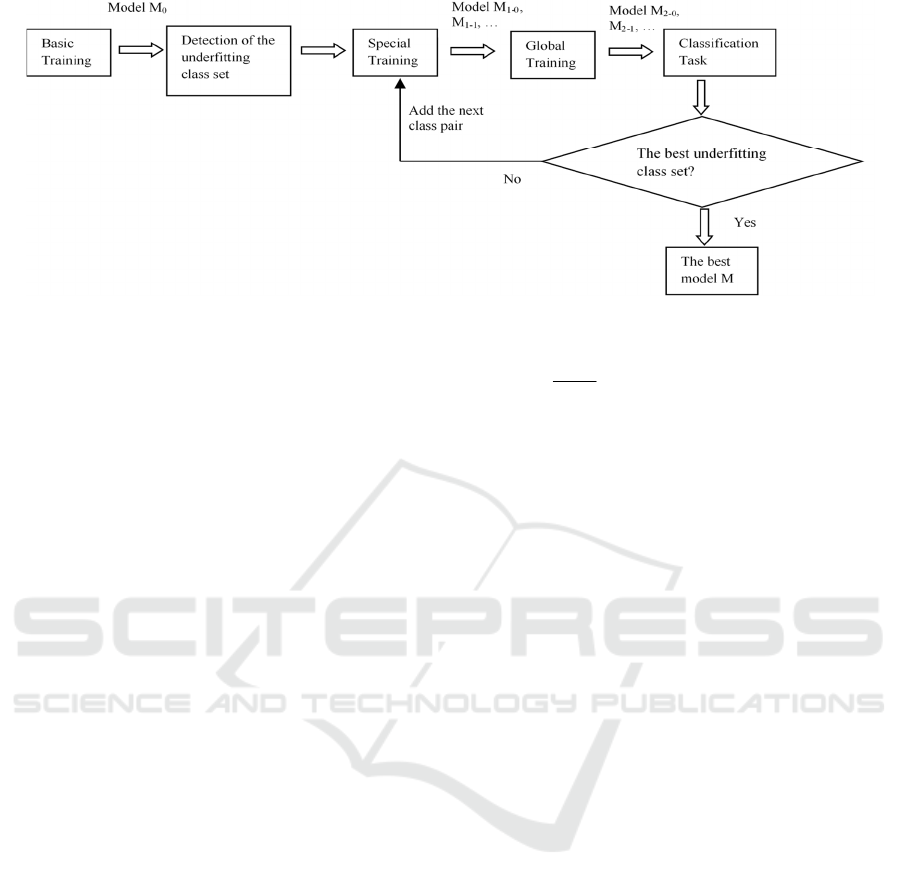
Figure 1: The procedure of the proposed method.
Many people have improved the results of neural
networks based on the interpretation conclusion.
Deconvolutional Network (Zeiler et al., 2011) was
used to visualize (Zeiler and Fergus, 2014) feature
maps in different layers, and they used visualization
result to debug problems of the model to get better
results. Ribeiro et al. (2016) extracted image regions
that are highly sensitive to the network output and
they improved the untrustworthy classifier in the
network they used. Yosinski et al. (2014) have
analyzed the transferability of intermediate
representation of each layer, and they found that
initializing with transferred features would improve
CNN performance. There is also a study (Zintgraf et
al., 2017) on visualizing areas in the input image that
contribute the most to the decision-making process of
CNN, which can help improve models. However,
these work mainly used the interpretation on CNN to
improve the classification result of networks. In this
paper, between-class distance is used to understand
the discrimination power of the trained model
between different classes, and then the analysis is
used to improve the training process, which provides
a new perspective for improving the effect of CNN.
3 THE PROPOSED METHOD
In this section, the proposed method which uses
between-class distances of the deep features to
improve the training is introduced.
3.1 Between-class Distance
In order to accurately evaluate the discrimination
power of the network, this paper uses an indicator
dist_bt, which shows the between-class distance. The
variable dist_bt is defined as:

11
1
,
nm
ij
ij
dist_bt Eu_distance A B
nm




(1)
where A and B refer to classes that contain n and m
objects respectively, A
i
, B
j
refer to feature maps
produced by the i-th object in class A and j-th object
in class B respectively, and function Eu_distance (A
i
,
B
j
) is to calculate the Euclidean distance between A
i
and B
j
. It can be seen that dist_bt represents the
average distance between class A and class B.
3.2 Improving the Training of CNN
When one needs to improve classification accuracy of
a network, a trial and error method may be the first
choice. But it will waste too much time. In this paper,
a new training approach is proposed to improve the
training of the network used in multi-class
classification tasks. Figure 1 provides a brief
introduction of the procedure which includes the
following steps:
(1) Basic training. First we need to train the data
on a CNN architecture and get model M
0
that includes
parameters of basic training. Here the data is divided
into training set, validation set, and test set.
(2) Detection of the underfitting class set. The
second step is to identify classes which are not trained
sufficiently in the basic training. A between-class
distance matrix is used to identify “underfitting
classes”. Validation set is used to control the training
epochs.
If the distance computed using the formula (1)
between two classes is small, it is difficult for the
network to distinguish between them.
So, the underfitting classes are selected from
ordered class pairs, such as (C
0
, C
1
), (C
1
, C
2
), …,
which are sorted by the between-class distances from
small to large. At first the class pair (C
0
, C
1
) with the
smallest between-class distance is selected to create
NCTA 2020 - 12th International Conference on Neural Computation Theory and Applications
362

the underfitting class set which is {C
0
, C
1
}, and then
the class pair (C
1
, C
2
) with the second smallest
between-class distance is added and a new
underfitting class set including {C
0
, C
1
, C
2
} is
produced. The next class pair in the ordered class
pairs is continuously added until the best underfitting
class set is found in step (4).
(3) Special training. This is the most crucial step.
We need to train the underfitting class set and the
training is based on the model M
0
trained in the basic
training. Data objects are randomly selected from the
classes in the underfitting class set, and the number of
the selected objects in each class is the same as that in
the basic training. Assuming that{C
0
, C
1
, C
2
} is the
underfitting class set, and the selected data objects
from the three classes are named as D
0
, D
1
and D
2
respectively. First, the dataset {D
0
, D
1
} is used as the
initial dataset on special training based on the model
M
0
, which result in a new model M
1-0
. Later, {D
0
, D
1
,
D
2
} will be used in the special training to produce a
new model M
1-1
based on M
0
. This process is continued
until the best underfitting class set is found in step (5).
(4) Global training. The difference between global
training and the special training is that the former uses
all the classes but the latter focuses on the underfitting
class set. The initial model for global training is
generated from the special training such as M
1-0
, M
1-
1
, etc. Both the training data and the hyper-parameters
used in this step are the same as that in the basic
training in step (1). After the global training, new
models named such as M
2-0
, M
2-1
, etc. are produced
from the models named M
1-0
, M
1-1
, etc.
(5) Identifying the best underfitting class set. To
find the best underfitting class set, the classification
accuracy on the validation set using the models, such
as M
2-0
, M
2-1
, …, produced by the global training are
computed. If the classification accuracy of a model
M
i
is higher than that of the model M
i+1
which is the
model produced by adding more classes to the
underfitting class set of M
i
, the model M
i
is identified
as the best model, and the corresponding underfitting
class set is identified as the best underfitting class set.
In the proposed method, the validation set plays
an important role, which is used to adjust the hyper-
parameters and to identify the best underfitting class
set.
4 EXPERIMENT AND ANALYSIS
In this section, the proposed method is mainly applied
on the MNIST dataset (Lecun and Bottou, 1998) and
the EMNIST dataset (Cohen et al., 2017) to evaluate
the performance.
4.1 Training Details
The network structure used in the experiments is
similar with LeNet-5. The only difference is that
Softmax is used as the output layer.
Adaptive moment estimation (Adam) with a batch
size of 128 was used to update the parameters.
Starting with 0.001, the learning rate is reduced every
300 steps with a decay rate of 0.4 throughout the
training. Dropout is used in the last full connected
layer with a rate of 0.7. Values of all the weights are
initialized to 10
-2
and biases are set to 0.
4.2 Improve the Classification
Accuracy on MNIST
The first dataset used is selected from MNIST
randomly. 3200 pictures are selected as the training set.
For both the validation set and the test set, 800 pictures
are selected for each of them. Since there are 10 classes
in the dataset, the number of pictures in each class in
the training set, the validation set and the test set is 320,
80 and 80 respectively. The experimental results on
MNIST are shown in the following.
First, the basic training has been done according
to the details described in Section 4.1 to get model M
0
.
The between-class distance matrix and the confusion
matrix computed after the basic training on the
validation set and the test set are showed in Figure 2
and Figure 3 respectively. It can be seen that the
results on the validation set are similar to the results
on the test set, and the confusion matrix is basically
consistent with the between-class distance matrix. For
example, it can be seen that class 4 and class 9, class
5 and class 8 are the two class pairs which has the
smallest between-class distances on both the
validation set and the test set. And it can be found that
class 4 and class 9, class 5 and class 8, class 5 and
class 3 are the three underfitting classes which have
the smallest between-class distances, while the
classes 5, 8, 9 have lowest classification accuracy as
shown in the diagonal of the confusion matrix on the
validation set.
During the special training, the data objects from class
4 and class 9 are randomly selected and set as the initial
training dataset. These data are trained for 100 epochs
based on M
0
to produce a new model M
1-0
. Then the
data from class 5 and class 8 are added into the initial
training dataset to produce the underfitting class set {4,
9, 5, 8} and are trained for 100 epochs based on M
0
to
get model M
1-1
. At last, the data from class 3 are added
to produce the underfitting class set {3, 4, 9, 5, 8},
which are trained for 100 epochs to produced the
corresponding model M
1-2
.
Improving the Training of Convolutional Neural Network using Between-class Distance
363

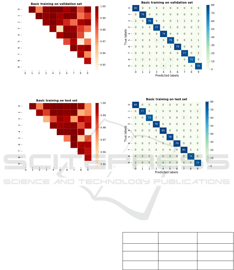
Figure 2: The left picture is the between-class distance matrix and the right one is the confusion matrix computed with the
model M
0
on the validation set of the MNIST dataset in the basic training.
Figure 3: The left picture is between-classes distance matrix and the right one is confusion matrix on the test set with the
model M
0
on the validation set of the MNIST dataset.
Using the same data and the parameters as in
basic training, the global training is done based on
model the M
1-0
, M
1-0
and M
1-2
. After training 200,
250, 300 epochs respectively, three improved
training models M
2-0
, M
2-1
and M
2-2
are generated.
For this dataset the best underfitting class set found
using the validation set is {4, 9, 5, 8}, So the best
model is
M
2-1.
The between-class distance matrix and the
confusion matrix calculated with the model M
2-0
, M
2-
1
and M
2-2
on the test set are shown in Figure 4. It can
be seen that the performance is greatly improved
compared to model M
0
in Figure 3 with the same
training data.
Table 1 shows the classification accuracy of these
models on the test set. For comparison, the method
called “the original training method” is refer to
simply train the original dataset by the number of
epochs equal to the total number of epochs used in the
basic training, the special training and the global
training in the proposed method.
Table 1: Comparison of the classification accuracy of the
proposed method and the original training method on the
MNIST dataset.
Model
The original
training metho
d
The proposed
metho
d
M
2-0
97.75 % 98.25%
M
2-1
97.25% 98.5%
M
2-2
97.25% 97.63%
It can be seen from Table 1 that the original
proposed method can effectively improve the training
method. The highest classification accuracy 98.5% is
produced on the model M
2-1
by the proposed method,
which is consistent with the best model found using
the validation set.
NCTA 2020 - 12th International Conference on Neural Computation Theory and Applications
364

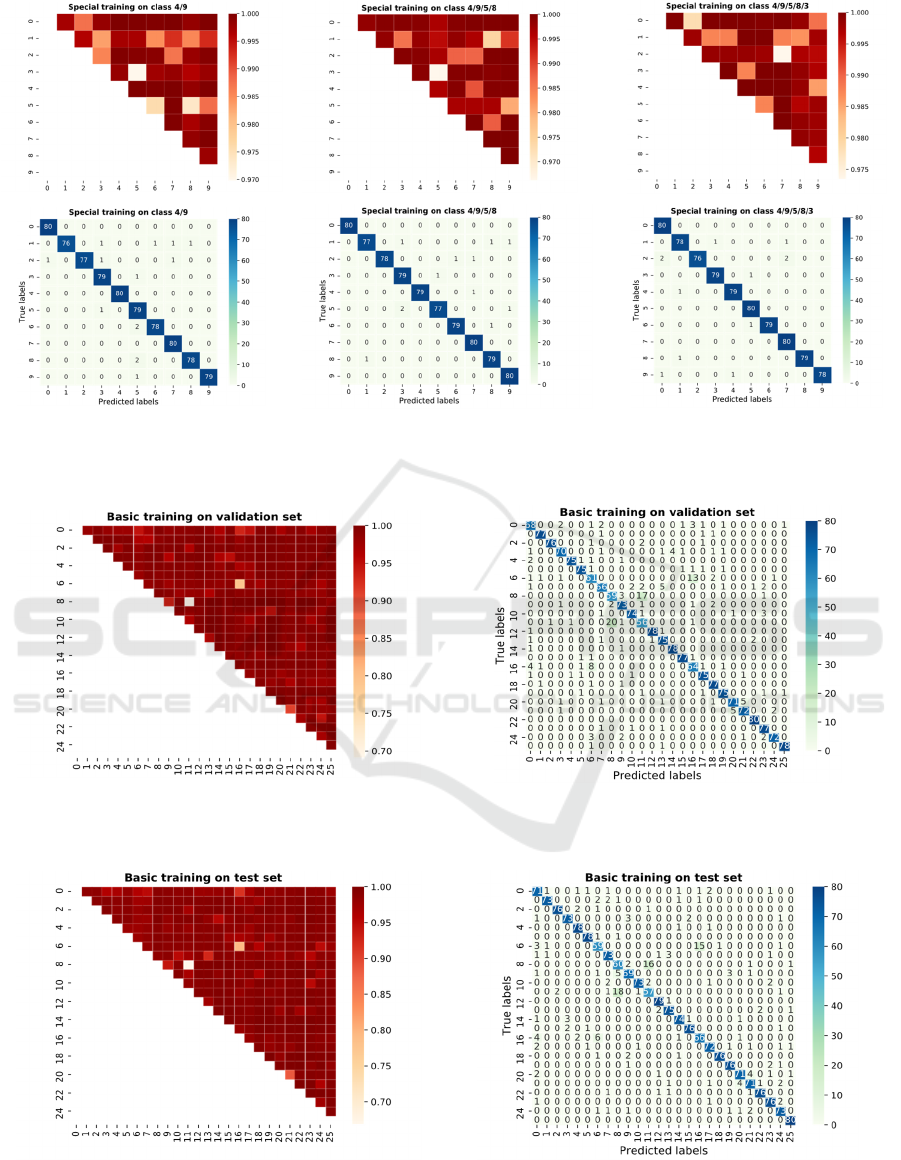
Figure 4: The first row shows the between-class distance matrix and the second row shows the confusion matrix on the test
set after both the special training and the global training. The three columns contain the results produced with model M
2-0
,
M
2-1
and M
2-2
respectively on the MNIST dataset.
Figure 5: The left picture is between-classes distance matrix and the right one is the confusion matrix on the validation set
in basic training for the EMNIST dataset.
Figure 6: The left picture is between-classes distance matrix and the right one is the confusion matrix on the test set in
basic training for the EMNIST dataset.
Improving the Training of Convolutional Neural Network using Between-class Distance
365

4.3 EMNIST
The EMNIST dataset is derived from NIST Special
Database 19. We mainly use Letters in EMNIST. The
way of data division used in this experiment is the
same with that in MNIST.
The between-class distance matrix and the
confusion matrix computed after the basic training on
the validation set and the test set are showed in Figure
5 and Figure 6 respectively. Classification accuracy
after the basic training is 90.43%. It can be found
from Figure 5 that class 8 and 11, class 6 and 16 are
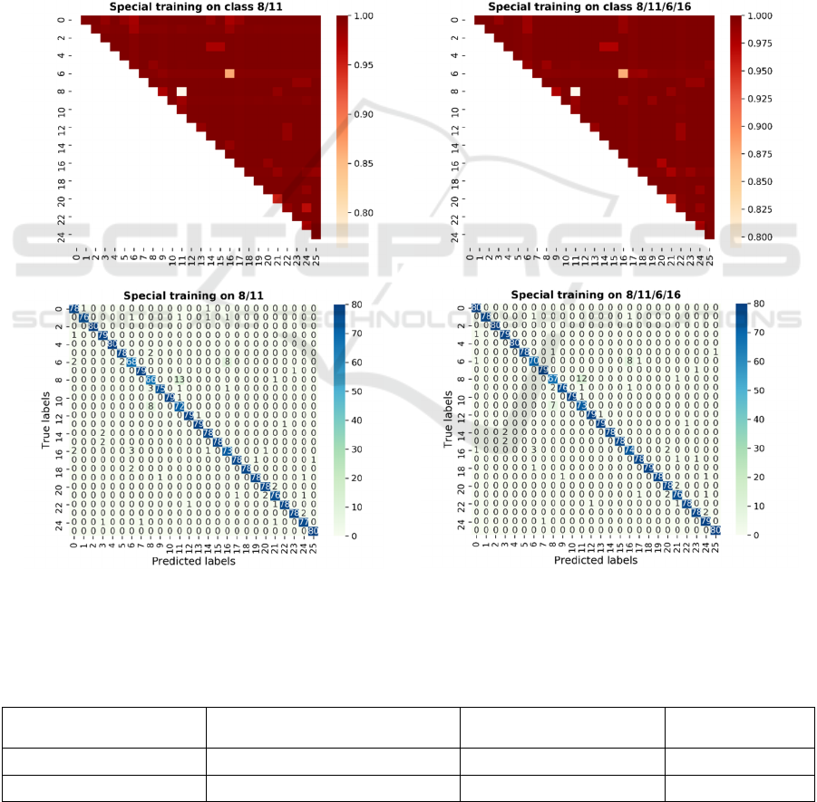
“underfitting classes”. So the corresponding special
training includes 2 steps: the first one is on classes 8
and 11, which results in a model M
1-0
, and the second
one is on the class set {8, 11, 6, 16}, which results in
a model M
1-1
. After the global training, we get a
model M
2-0
and a model M
2-1
. The result of the global
training is shown in Figure 7. It is obvious that value
between underfitting classes in confusion matrix are
smaller, and data in between-class distance matrix
becomes larger compared with that in Figure 6. Table
2 shows that the classification accuracy produced by
the proposed method is higher than that of the original
training method. In this experiment, the best model is
M
2-1
, and the best underfitting class set is {8, 11, 6,
16}.
Figure 7: The first row shows the between-class distance matrix and the second row shows the confusion matrix on the test
set after both the special training and the global training. The two columns contain the results produced with model M
2-0
an
d
model M
2-1
res
p
ectivel
y
on the EMNIST dataset.
Table 2: Comparison of the classification accuracy of the proposed method and the original training method on the EMNIST
dataset.
Model
#Epoches in Special Training/
Global Training
The original training
method
The proposed
method
M
2-0
500/500 90.53% 91.13%
M
2-1
500/1000 90.58% 91.20%
NCTA 2020 - 12th International Conference on Neural Computation Theory and Applications
366

5 CONCLUSION
In this paper, we propose a new method to improve
the training process in multi-class classification using
CNN. The method proposed in this paper is different
from training with random parameter adjustment, but
based on the actual properties of the feature maps
after the basic training. Between-class distance is
used in this paper to find the specific classes that are
not trained sufficiently in the basic training. Then
additional training processes are used to deal with the
insufficient training problem. It is found that the
between-class distances computed on the learned
feature maps can be used to improve the network
training. In the future, we will test whether the
proposed method is practical on more sophisticated
networks and larger datasets.
ACKNOWLEDGEMENTS
This work is supported by the National Key R&D
Program of China (Grants No. 2017YFE0111900,
2018YFB1003205).
REFERENCE
Lecun, Y. , Boser, B. , Denker, J. , Henderson, D. , Howard,
R. , & Hubbard, W. , et al. (1989). Backpropagation
applied to handwritten zip code recognition. Neural
Computation, 1(4), 541-551.
Lecun, Y. , & Bottou, L. . (1998). Gradient-based learning
applied to document recognition. Proceedings of the
IEEE, 86(11), 2278-2324.
Krizhevsky, Alex, Sutskever, Ilya, Hinton, Geoffrey E.
Advances in Neural Information Processing Systems, v
2, p 1097-1105, 2012
Deng, J., Dong, W., Socher, R. , Li, L. J. , & Li, F. F. . (2009).
ImageNet: A large-scale hierarchical image database.
IEEE Conference on Computer Vision & Pattern
Recognition. IEEE.
Szegedy, C. , Liu, W. , Jia, Y. , Sermanet, P. , Reed, S. , &
Anguelov, D., et al. (2014). Going deeper with
convolutions.
Simonyan, K. , & Zisserman, A. . (2014). Very deep
convolutional networks for large-scale image
recognition. Computer ence.
Huang, G. , Liu, Z. , Laurens, V. D. M. , & Weinberger, K.
Q. (2017). Densely connected convolutional networks.
Gerardo Hernández, Zamora, E. , Sossa, H. , Germán Té
llez, & Federico Furl á n. (2019). Hybrid neural
networks for big data classification. Neurocomputing.
Ren, S. , He, K. , Girshick, R. , & Sun, J. . (2017). Faster r-
cnn: towards real-time object detection with region
proposal networks. IEEE Transactions on Pattern
Analysis & Machine Intelligence, 39(6), 1137-1149.
Dai, J., Li, Y., He, K., & Sun, J. (2016). R-FCN: Object
Detection via Region-based Fully Convolutional
Networks. NIPS.
He, K. , Gkioxari, G. , Piotr Dollár, & Girshick, R. . (2017).
Mask R-CNN. 2017 IEEE International Conference on
Computer Vision (ICCV). IEEE.
Er, M. J. , Zhang, Y. , Wang, N. , & Pratama, M. . (2016).
Attention pooling-based convolutional neural network
for sentence modelling. Information ences An
International Journal.
Zhang, Q. S. , & Zhu, S. C. . (2018). Visual interpretability
for deep learning: a survey. Frontiers of Information
Technology & Electronic Engineering, 19(01), 27-39.
Zeiler, M. D. , & Fergus, R. (2014). Visualizing and
Understanding Convolutional Networks. European
Conference on Computer Vision. Springer, Cham.
Mahendran, A. , & Vedaldi, A. . (2014). Understanding deep
image representations by inverting them.
Bau, D., Zhou, B., Khosla, A., Oliva, A., & Torralba, A.
(2017). Network Dissection: Quantifying
Interpretability of Deep Visual Representations. 2017
IEEE Conference on Computer Vision and Pattern
Recognition (CVPR), 3319-3327.
Zhang, Q. , Cao, R. , Shi, F. , Wu, Y. N. , & Zhu, S. C. .
(2017). Interpreting cnn knowledge via an explanatory
graph.
Yosinski, J. , Clune, J. , Bengio, Y. , & Lipson, H. . (2014).
How transferable are features in deep neural networks?.
International Conference on Neural Information
Processing Systems. MIT Press.
Zintgraf, L. M. , Cohen, T. S. , Adel, T. , & Welling, M. .
(2017). Visualizing deep neural network decisions:
prediction difference analysis.
Lakkaraju, H., Kamar, E., Caruana, R., & Horvitz, E. (2017).
Identifying Unknown Unknowns in the Open World:
Representations and Policies for Guided Exploration.
AAAI.
Ribeiro, M. T. , Singh, S. , & Guestrin, C. . (2016). "why
should i trust you?": explaining the predictions of any
classifier.
Zhang, Q. , Yang, Y. , Ma, H. , & Wu, Y. N. . (2019).
Interpreting cnns via decision trees.
Fergus, R. , Taylor, G. W. , & Zeiler, M. D. . (2011).
Adaptive deconvolutional networks for mid and high
level feature learning. International Conference on
Computer Vision. IEEE Computer Society.
Cohen, G. , Afshar, S. , Tapson, J. , & Schaik, A. V. . (2017).
EMNIST: Extending MNIST to handwritten letters.
International Joint Conference on Neural Networks.
IEEE.
Improving the Training of Convolutional Neural Network using Between-class Distance
367