Ontology-based Processing of Dynamic Maps in Automated Driving

Haonan Qiu

1,2

, Adel Ayara

and Birte Glimm

BMW Car IT GmbH, Ulm, Germany

Institute of Artiﬁcial Intelligence, University of Ulm, Germany

Keywords:

Autonomous Driving, Digital Maps, Ontologies, Rules, Knowledge Representation.

Abstract:

Autonomous cars act in a highly dynamic environment and consistently have to provide safety and comfort

to the passengers. For a car to understand its surroundings, a detailed, high-deﬁnition digital map is needed,

which acts as a powerful virtual “sensor”. Compared to traditional digital maps, high-deﬁnition maps require

signiﬁcantly more storage space, which makes it largely impossible to store a complete map in a navigation

system. Furthermore, map data is provided in numerous heterogeneous formats. Consequently, interoper-

ability and scalability have become the main challenges of existing map processing solutions. We address

these challenges by providing an interoperable knowledge-spatial architecture layer based on ontologies and

conﬁrm the scalability in an empirical evaluation.

1 INTRODUCTION

In 1990, a digital map was used for the ﬁrst time

in a built-in GPS-based navigation system offered

by Mazda Eunos Cosmos cars (Leite, 2018). In the

2000s, great effort has been made to develop en-

hanced digital maps for supporting Advanced Driver

Assistance Systems (ADAS). Enhanced digital maps

are low-resolution maps containing road geometry

and road attributes, such as road width and speed limit

for ADAS at road level. We refer to enhanced digital

maps as standard deﬁnition (SD) maps. Autonomous

vehicles need, however, maps with a higher level of

detail than what SD maps typically offer. In 2010,

the concept of a “high-deﬁnition map” was introduced

during a research workshop and such maps were then

used in 2013 in the Bertha Drive Project (Herrtwich,

2018).

In contrast to SD maps, high-deﬁnition (HD) maps

provide detailed information at lane level to support

vehicle perception and localisation (Gruyer et al.,

2016). Based on the functional system architecture of

an automated driving system by Ulbrich et al. (2017),

HD maps with localisation functionality provide in-

puts to the perception module for world modelling,

and eventually support the decision making of the

planning and control module. Almost all players in

the area of highly automated driving, e.g., Google,

HERE, TomTom, Baidu, BMW, or Toyota, rely on

HD maps to further improve the driving capabilities

of their autonomous vehicles.

Recently, collective efforts have been made to-

wards standardising HD maps, such as Geographic

Data File (GDF) 5.1 at international level (ISO/TC

204, 2018) or Navigation Data Standard (NDS) and

the ADASIS protocol V3 at industrial level (NDS

Association, 2018). There are also national efforts

for developing HD map standards, such as the China

Industry Innovation Alliance for the Intelligent and

Connected Vehicles (CAICV). However, as of now,

there is no single, authoritative format or standard

for HD maps. As a result, map model development,

maintenance, and integration, as well as map data ex-

change and sharing pose major challenges in practise.

HD maps are extremely detailed and, therefore,

require signiﬁcantly more processing power and com-

putation resources compared to SD maps. This makes

it largely impossible to store a complete detailed map

within a vehicle’s navigation system. Hence, the nav-

igation system needs to constantly request map data

streams while the car is progressing along a route and

care has to be taken to provide any relevant informa-

tion in time.

Summing up, the characteristics of HD maps re-

quire a novel approach that allows for a generic repre-

sentation of the road environment and a dynamic up-

date mechanism. Ontology-based road environment

modeling has gained growing interest for this pur-

pose in the Intelligent Transportation Systems com-

munity (Katsumi and Fox, 2018; Chen and Kloul,

Qiu, H., Ayara, A. and Glimm, B.

Ontology-based Processing of Dynamic Maps in Automated Driving.

DOI: 10.5220/0010133900980107

In Proceedings of the 12th International Joint Conference on Knowledge Discovery, Knowledge Engineering and Knowledge Management (IC3K 2020) - Volume 2: KEOD, pages 98-107

ISBN: 978-989-758-474-9

2018; Bagschik et al., 2018), e.g., for road models that

provide different features for speciﬁc application re-

quirements (Zhao et al., 2017; Armand et al., 2017)

and for spatial knowledge representation and reason-

ing for navigation and path planning (Belouaer et al.,

2010; Hudelot et al., 2008).

In this paper, we address the challenge of dynam-

ically updating the map data used within the naviga-

tion system of autonomous vehicles. The main con-

tributions are as follows:

– We propose a knowledge-spatial architecture,

based on OWL 2 RL ontologies (Hitzler et al.,

2009), Datalog rules (Abiteboul et al., 1995),

and SPARQL queries (W3C SPARQL Work-

ing Group, 2013), to deal with both knowledge

abstraction and spatial reasoning on map data

streams.

– We present a categorisation of the types of rules

that are needed for knowledge abstraction and

spatial reasoning.

– We propose the use of spatial window queries for

continuous knowledge updates. Spatial windows

contain an object, if the object satisﬁes a certain

spatial query.

– We evaluate the approach for dynamic map up-

dates in a high way scenario within our prototype

called SmartMapApp.

The remainder of this article is structured as follows:

First, we present some background knowledge about

map data concepts and ontological modelling in Sec-

tion 2. In Section 3, we introduce the knowledge-

spatial architecture in detail. In Section 4, we evaluate

the approach. We then brieﬂy discuss the designing

choices between SPARQL and Datalog in Section 5.

Finally, we give conclusion in Section 6.

2 PRELIMINARIES

In this section, we ﬁrst brieﬂy describe the map data

model. Then we provide an introduction to ontolo-

gies, rules and SPARQL.

2.1 Map Data

Conceptually, HD maps mainly contain three layers:

the road model, the lane model, and the localisation

model, while SD maps only cover the road model.

The road and the lane model layers are very impor-

tant since they contain the semantics of the road and

lane segments. The road model contains parts of the

road that are not part of the lanes, such as edges of the

road. It uses an ordered sequence of shape points that

describe the geometry of a polyline in the direction of

the road. Each road segment has a start and an end

node, which belong to the intersection at the start and

end of the road.

However, since autonomous vehicles are designed

to center themselves in the lane, in reality, au-

tonomous vehicles only need to deal with the lane

model except on rare occasions when they need to

travel outside the lane boundaries. The lane model

includes information on lane geometries (boundaries,

width, curvature, etc.), lane connectivity, lane type

(vehicle lane, exit lane, etc.), travel direction, lane

marking types (solid/dashed, single/double. etc.), and

speed limits. The lane geometry determines the accu-

racy, storage efﬁciency and usability of the HD maps

(Gwon et al., 2017). We refer the interested reader to

the literature for further details about HD maps (Liu

et al., 2020; Gran, 2019).

In practise, different companies provide maps in

their own format and structure. Table 1 shows exam-

ples of the differences between two HD map formats,

namely the HERE map content format and the NDS

format. The ﬁrst two columns show the differences

in naming conventions, while the later two columns

show the differences in deﬁnitions.

2.2 Ontologies

Studer et al. (1998) deﬁne an ontology as a “a formal,

explicit speciﬁcation of a shared conceptualization”.

More concretely, an ontology describes concepts and

relations that are relevant to the modeling of a do-

main of interest. The three main building blocks of

an ontology are: 1) Classes (aka concepts), which are

representations of the concepts of the domain that the

ontology aims to describe (e.g., Lane); 2) Individu-

als, which represent concrete entities in the applica-

tion domain (e.g., lane1); 3) Properties, which repre-

sent attributes of and relationships between individu-

als (e.g., hasLength or hasDirectLeft). Properties are

divided into object and data properties. Object prop-

erties are binary relationships between two individu-

als, while data properties relate individuals to literal-

s/concrete data values (e.g., an integer value). Finally,

an ontology is a set of axioms, i.e., general statements

(e.g., stating that LeftMostLane is a subclass of Lane)

and concrete facts (e.g., hasDirectLeft(lane1, lane2) or

Lane(lane1)) about the application domain described

using classes, properties and individuals.

The Web Ontology Language (OWL) is a for-

mal language designed to model complex knowledge.

OWL 2 RL is a fragment (aka proﬁle) of OWL de-

signed for handling large amounts of data/facts, where

Ontology-based Processing of Dynamic Maps in Automated Driving

Table 1: Examples of differences in HD map formats.

Point Road Part Numbering of Lanes Lane Forming/Ending

HERE node segment left to right #lanes changes

NDS shape point link curbside to middle #lanes changes & physically separated

implicit facts can be derived via rule-based reason-

ing. Ontologies can be speciﬁed using the Resource

Description Framework (RDF), where the axioms

are written as subject-predicate-object triples using

IRIs, blank nodes (representing existentially quanti-

ﬁed variables) and literal values. For example, the fact

Lane(lane1) is written as :lane1 rdf:type :Lane in RDF

assuming suitable preﬁx declarations for the IRIs.

2.3 Rules

Rules can be used to axiomatise the semantics of a

particular Web ontology language, e.g., OWL 2 RL,

via a static set of rules or, using datalog rules, users

can create custom rule sets. In order to deﬁne datalog

rules, we ﬁx countable, disjoint sets of constants and

variables. A term is a constant or a variable. An atom

has the form P(t

,... ,t

), where P is a k-ary predi-

cate and each t

, 1 ≤ i ≤ k, is a term. We focus on

unary and binary atoms only (i.e., 1 ≤ k ≤ 2), which

correspond to classes and properties of the ontology,

respectively. An atom is ground if it does not contain

variables. A fact is a ground atom and a dataset is

a ﬁnite set of facts, e.g., as deﬁned in an ontology.

A datalog rule is a logical implication of the form

,. .. ,H

← B

,. .. ,B

, where each H

, 1 ≤ i ≤ j, is

a head atom, and each B

, 1 ≤ ` ≤ k, is a body atom.

A datalog program is a ﬁnite set of rules. The con-

sequents (head) of the rule are true, if all body atoms

of a rule are true. The main computational problem

in datalog systems is answering queries over the facts

that logically follow from the explicitly stated facts

and a datalog program.

A negative body atom has the form, NOT EXISTS

, . . . , v

IN B, where each v

, 1 ≤ i ≤ j, is a vari-

able and B is an atom. A rule r is safe if variables that

appear in the head or in a negative body atom also

appear in a positive body atom. A safe datalog rule

can be extended with stratiﬁed negation by extend-

ing the rule to have negative body atoms, where there

is no cyclic dependency between any predicate and a

negated predicate.

An aggregate is a function that takes a multi-

set of values as input and returns a single value

as output. An aggregate atom has the form

Aggregate(B

,. .. ,B

ON x

,. .. ,x

BIND f

) AS

.. . BIND f

) AS r

), where each B

, 1 ≤ i ≤ k, is

an atom, each x

, 1 ≤ u ≤ j, is a variable that appears

in B

, each f

, 1 ≤ v ≤ n, is an aggregate function,

each e

, 1 ≤ w ≤ n, is an expression containing vari-

ables from B

, and each r

, 1 ≤ z ≤ n, is a constant for

a variable that does not appear in B

2.4 SPARQL

SPARQL is a query language for RDF graphs based

on pattern matching. For example, the query

SELECT ? l WHERE

{ ? l rd f : type : L e f t M o st L a n e }

selects all individuals that are instances of the class

:LeftMostLane. Note that we omit preﬁx declara-

tions and we assume the queries to be evaluated over a

pre-deﬁned dataset in an RDF datastore. SPARQL 1.1

is the latest version supporting subqueries, value as-

signment, path expressions, aggregates, negation via

FILTER NOT EXISTS and derivation of RDF nodes

via BIND (W3C SPARQL Working Group, 2013). It

also provides operations that update, create and re-

move data.

2.5 SKOLEM

Skolem functions allow dynamically generate “fresh"

IRIs for blank nodes, called Skolem IRIs. Sys-

tems use Skolem IRIs “should mint a new, globally

unique IRI (a Skolem IRI) for each blank node so

replaced."(Cyganiak et al., 2014) The Skolem func-

tion takes the form as SKOLEM("s", v

,. .. ,v

), where

s is a arbitrary string and each v

, 1 ≤ i ≤ k, is a

variable appearing in the rule body. Skolem IRIs

are implemented using hasing schemes of various

lengths (Hogan, 2015). BIND function assgins the

Skolem IRI to an new variable. It takes the form

as BIND(SKOLEM("s", v

,. .. ,v

) AS n), where n is the

new variable holds the Skolem IRI.

3 A KNOWLEDGE-SPATIAL

ARCHITECTURE

In this section, we present the knowledge-spatial ar-

chitecture that enables autonomous vehicles to per-

ceive their environment with a dynamic map. We then

explain the two-level ontologies and related rules pat-

terns for knowledge abstraction and discuss how spa-

tial reasoning interacts with knowledge abstraction.

KEOD 2020 - 12th International Conference on Knowledge Engineering and Ontology Development

100

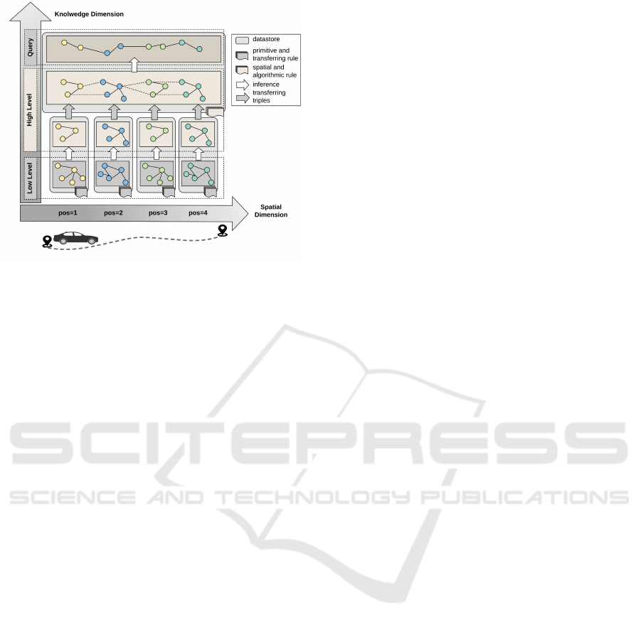
Figure 1: The overview of knowledge-spatial architecture.

3.1 Architecture Overview

Figure 1 depicts the overall knowledge architec-

ture. Inspired by the Global Ontology Approach

(Wache et al., 2001), we perform a knowledge ab-

straction process across the knowledge dimension

(vertical axis) from the format-speciﬁc and detailed

low-level ontologies to the generic high-level on-

tology. The horizontal (time) axis represents road

knowledge acquisition events, which trigger the

knowledge abstraction process via spatial reasoning.

Spatial reasoning considers updated vehicle motion

events determined in the knowledge abstraction pro-

cess and searches for spatial patterns to derive the rel-

evant consequences of what is happening on the road.

Different low-level ontologies for the different map

formats can be used to feed the high-level ontology,

which makes the proposed architecture very ﬂexible

as application-oriented queries, such as ADAS func-

tions, are posed over the generic high-level ontology

(Suryawanshi et al., 2019; Qiu et al., 2020).

The spatial dimension is orthogonal to the knowl-

edge dimension and correlates facts that are true

within a certain space. It describes the continu-

ous spatial reasoning process with respect to the up-

dated vehicle position and dynamic road environmen-

tal knowledge. We adopt the notion of a spatial win-

dow with a ﬁxed width or region in terms of a geo-

graphic element shift (slide) over a path line. Inspired

by Mokbel et al. (2005), we use the notion of spatial

expiration depending on the spatial location of a mov-

ing object, e.g., a vehicle, and stored data expires only

when the object leaves the spatial window.

Location-aware environments are, by nature,

highly dynamic and the size of spatial streams is po-

tentially inﬁnite. To deal with this challenge, certain

spacial events (e.g., the available map foresight of the

vehicle reaches a threshold) trigger the initialisation

of a new datastore for a low-level ontology. The next

map data region is loaded (as deﬁned by the speciﬁc

map data format) and used to generate more abstract,

high-level knowledge. While the high-level datastore

uses spatial expiration for deletions, a low-level data-

store is discarded once the high-level datastore is pop-

ulated.

3.2 Rule Classiﬁcation

Rules play a key role for knowledge abstraction and

spatial reasoning. The main challenges for rule mod-

elling are to (1) enrich instances at the primitive level;

(2) transfer low-level ontologies with different con-

cept deﬁnitions to a uniﬁed high-level ontology; (3)

derive spatial relations for spatial reasoning; (4) cap-

ture decision-making algorithms in rules.

Based on the challenges mentioned above, we

classify rules into (1) primitive, (2) transfer, (3) spa-

cial and (4) algorithmic rules and we describe the four

categories with sub-categories, examples and more

formal rule patterns below. In the formal patterns,

we use (possibly with subscripts) C for classes, op

for object properties, and dp for data properties of the

ontology over which the rules are to be executed.

3.2.1 Primitive Rules

These rules enrich instances with one-step inferences

and their results serve as input for all other rules.

Primitive rules use the identiﬁers to infer the relation-

ships or attributes and are divided into primitive rela-

tionship rules and primitive attribute rules.

(a) Primitive relationship rules infer relationships be-

tween individuals. For a concrete example consider:

hasLane(x, y) ← RoadPart(x), hasIdx(x, i),

Lane(y), hasIdx(y,i).

More generally, such rules have the form

op(x, y) ← C

(x), dp(x, z), C

(y), dp(y,z)

(b) Primitive attribute rules infer an attribute of an in-

dividual. For a concrete example consider:

speed(x, v) ← Node(x), hasIdx(x, i),

speedVal(y,v), hasIdx(y,i).

More generally, such rules have the form

dp(x, v) ← C(x), dp

(x, z), dp

(y, v), dp

(y, z).

Ontology-based Processing of Dynamic Maps in Automated Driving

101

3.2.2 Transfer Rules

These rules create a new individual in one ontology

(typically the high-level ontology) based on one or

more individuals in another ontology (typically a low-

level ontology). SKOLEM functions and string ma-

nipulations are used to dynamically generate named

(not anonymous) individuals (Shaw et al., 2011). The

rules are further divided into simple (1:1) and complex

(n:1) transfer rules according to instance correspon-

dence.

(a) Simple rules create, for each individual of a cer-

tain type in one ontology, a new individual of a cer-

tain type in another ontology. For a concrete example,

consider:

RoadPar t(r), hasPoint(r, s), length(r,l) ←

Link(k), hasShapePoint(k,s),

length(k, l), BIND(SKOLEM("rp", k) AS r).

More generally, such rules have the form

(n), op

(n,u), dp

(n,v) ←

(x), op

(x, u), dp

(x, v),

BIND(SKOLEM("c", x) AS n),

where C

, op

, and dp

are from one ontology and C

, and dp

are from another ontology.

(b) Complex rules create a new individual in one on-

tology based on several individuals in another ontol-

ogy and, hence, perform an aggregation process. As

a concrete example, consider the rule

Lane(l) ← Lane(l

), Lane(l

laneNum(l

,n), laneNum(l

,n),

hasConn(l

,c), hasConn(l

,c),

BIND(SKOLEM("l", c) AS l).

More generally, such rules have the form

(w) ← C

(x), C

(y),

(x, v), dp

(y, v),

(y, z), op

(y, z),

BIND(SKOLEM("c", z) AS w).

3.2.3 Spatial Rules

These rules infer important road environmental

knowledge for vehicle navigation (Gayathri and V.,

2018). We further subdivide them into bounding

rules, topological rules and distance rules.

(a) Bounding rules infer the boundaries of an area or

the range of a line, such as a start/end point or the left

or right-most lane. Aggregation functions (e.g., MIN

or MAX) can be used to identify an individual with a

minimal or maximal bounding value. As a concrete

example, consider:

LeftMostLane(z) ← Lane(p),

AGGREGATE(hasIdx(p, idx)

ON p BIND MAX(idx) AS m),

Lane(z), hasIdx(z, m).

More generally, such rules have the form

(z) ← C

(x), AGGREGATE(dp

(x, v) ON x

BIND MAX(v) AS m), C

(z), dp

(z,m).

Such rules might also use (stratiﬁed) negation to

identify individuals without some properties:

EndLane(x) ← Lane(x), NOT EXISTS y IN

(Lane(y), hasNext(x, y))

More generally, such rules have the form

(x) ← C

(x), NOT EXISTS y IN (C

(y), op

(x, y)).

(b) Topological rules refer to topological relations,

more speciﬁcally, lateral (left/right) and longitudinal

(predecessor/successor) relations. Reachability can

naturally be expressed using recursive rules.

hasLeft(x, y) ← hasDirectLeft(x,y)

hasLeft(x, z) ← hasDirectLeft(x,y), hasLeft(y,z).

More generally, such rules have the form

(x, y) ← op

(x, y)

(x, z) ← op

(x, y), op

(y, z)

objects, such as the distance to a point of interest.

There are two types of distance relations: coordinate

distance and length distance.

Coordinate distance rules indicate the distance

between two points using coordinates. An auxiliary

concept (CoordinateDistance) represents the ternary

relation that connects the source point to the target

point via two object properties hasSource and

hasTarget and the calculated distance value via the

data property distance:

CoordinateDistance(d), hasSource(d, s),

hasTarget(d,t), distance(d, z) ←

Point(s), x(s,x

), y(s, y

Point(t), x(t,x

), y(t, y

BIND(sqrt((x

− x

)

+(y

− y

)

) AS z),

BIND(SKOLEM("d", s, t) AS d).

More generally, such rules have the following form,

where A represents the auxiliary concept:

A(d), hasSource(d, s),

hasTarget(d,t), distance(d, z) ←

(s), x(s, x

), y(s, y

(t), x(t, x

), y(t, y

BIND(sqrt((x

− x

)

+(y

− y

)

) AS z),

BIND(SKOLEM("d", s, t) AS d).

KEOD 2020 - 12th International Conference on Knowledge Engineering and Ontology Development

102

Length distance rules are similar to coordinate

distance rules, but the distance is calculated by

aggregating the length of intermediate path elements

between two points. As a concrete example consider:

LengthDistance(d), hasSource(d, s),

hasTarget(d,t), distance(d, z) ←

Lane(s), length(s, v),

AGGREGATE(hasNext(s, p), hasNext(p,t)),

length(p, l) ON s BIND SUM(l) AS u),

BIND((v + u) AS z),

BIND(SKOLEM(" f ", s, t) AS d).

More generally, such rules have the form

A(d), hasSource(d, s),

hasTarget(d,t), distance(d, z) ←

(s), length(s, v),

AGGREGATE(op

(s, p), op

(p,t)),

length(p, l) ON s BIND SUM(l) AS u),

BIND((v + u) AS z),

BIND(SKOLEM(" f ", s, t) AS d).

3.2.4 Algorithmic Rules

These rules are used for decision making and vehi-

cle motion planning, e.g., for determining the most

probable path that a vehicle will take, for providing

lane-change notiﬁcations and for pre-fetching tiles.

The rules are modelled as a combination of rules of

different type, possibly requiring a speciﬁc rule order

(Suryawanshi et al., 2019; Qiu et al., 2020).

3.3 Knowledge Dimension: Two Levels

of Ontologies

To performance a knowledge abstraction process,

there are three main components involved, namely

low-level ontologies, a high-level ontology and rules.

The low-level ontologies represent the different map

data formats. The primitive rules produce the basic

semantics of instances at the low level. These ba-

sic semantics are the fundamental ingredients for the

transfer rules, which generate instances in the deﬁned

high-level ontology. The high-level ontology repre-

sents a generic and uniﬁed road environment model.

Spatial and algorithmic rules are used to reason over

the high-level ontology and provide the necessary

knowledge for decision making and vehicle motion

planing.

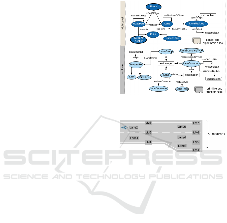
Figure 2 shows some of the concepts and rela-

tions of the high-level ontology and a low-level on-

tology representing HD map data based on the NDS

speciﬁcation. A LaneGroup is a set of one or more

lanes on a part of a link. A Lane is connected to

another lane via a LaneConnector. A LaneBound-

Figure 2: Overview of the two levels of ontologies for rep-

resenting map data; hasNBLane stands for hasNeighbour-

ingLane; hasLeftLM stands for hasLeftLaneMarking.

Figure 3: An example of a segment of a road and its lanes

and lane markings (LM).

ary is a line that separates lanes with type and colour

information. The corresponding high-level concepts

of Lane and LaneBoundary are Lane and LaneMark-

ing, respectively, and the instances of both concepts

are generated through low-level instances. The corre-

sponding high-level concept of Link is RoadPart and

its instances are generated through the instances of

Link. At the high level, the spatial relations among

Lane and RoadPart are essential for maintaining dy-

namic high-level road environmental knowledge (see

Figure 3). Figure 4 is a graph representation of the

example shown in Figure 3.

3.4 Spatial Dimension

With the volume and velocity of map data streams,

it becomes infeasible to store and process all avail-

able information. Hence, only some portion of the

available knowledge is stored in memory and only for

a limited area. The choice of the stored knowledge

is primarily dependent on continuous spatial queries.

In addition, we adopt a mechanism to expire (delete)

some of the stored knowledge and add information

relevant to answer decision-making queries. In our

approach, we employ a spatial window policy, where

Ontology-based Processing of Dynamic Maps in Automated Driving

103

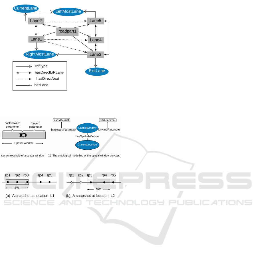
Figure 4: An example of Lane and RoadPart spatial rela-

tions; hasDirectL/RLane stands for hasDirectLeft/RightLane

corresponding to Figure 3.

Figure 5: Modelling of the spatial window.

Figure 6: A example of the spatial window (sw) with re-

spect to locations.

the spatial window is deﬁned as a range of an area

that satisﬁes some spatial properties (e.g., distance)

with respect to a reference object. We use spatial

rules, namely topological and distance rules, to per-

formance spatial reasoning.

The spatial window is relevant to the vehicle loca-

tion with the forward and backward parameters (see

Figure 5 (a)). It is modelled as a class SpatialWin-

dow with two data properties forwardParameter and

backwardParameter (see Figure 5 (b)). We deﬁne the

inside object property of a road part and a spatial win-

dow using the rule

inside(r, s) ←

RoadPar t(r), distanceToVehicle(r, d),

currentLocation(c), hasSpatialWindow(c, s),

SpatialWindow(s), forwardParameter(s, f ),

backwardParameter(s,b),

FILTER(d ≤ f && d ≤ b)

The SPARQL query

SELECT ? r WHERE {

? r rdf : t ype : Road P a r t .

? r : i n s i d e : S p at i a lW i n d o w .

}

then retrieves road parts that are inside a speciﬁc Spa-

tialWindow instance.

Figures 6 (a) and (b) give two snapshots of the

vehicle environment at the locations L1 and L2. The

objects labelled rp1 – rp5 represent road parts. At the

location L1, continuous spatial queries are evaluated

over rp1 – rp3 as they are inside the spatial window.

At location L2, however, r1 – r2 move out of the spa-

tial window, which means that they are expired. rp3 is

a still valid object and rp4 is the new object inside the

spatial window. Thus, the continuous spatial queries

are evaluated over rp3 and rp4.

4 EVALUATION

In this section, we evaluate the adequacy of the pro-

posed knowledge-spatial architecture in our proto-

type called SmartMapApp. The prototype uses RD-

Fox (Oxford Semantic Technologies, 2019) for stor-

ing, querying, and reasoning over map data. Then,

we present the experimental results for the knowledge

abstraction and for the spatial reasoning process.

4.1 Use Case

In order for an autonomous vehicles to navigate safely

and to ensure the comfort and safety of its passengers,

the navigation system needs to constantly request map

data streams while the vehicle is progressing along

a route. To achieve this goal, the Advanced Driving

(AD) system runs a continuous spatial query over the

incrementally updated road environmental knowledge

to check if the system needs to pre-load map data or

delete expired road entities. The concrete scenario is

described as following.

The vehicle initialises its world view with some

low-level map data, which results in a high-level road

view. As soon as the car starts to move, it triggers a

continuous pre-fetching query with a spatial window

whose forward parameter is set to 5 km. Afterwards,

the system pre-loads data for a new map tile based on

the answer of pre-fetching query. Consequently, the

high-level road view is extended with the new spatial

knowledge. While the system incrementally updates

the road environmental knowledge, it also continu-

ously checks if any road parts are “out of window"

based on the backward parameter (e.g., 3 km) of the

spatial window. The road parts which are no longer

“inside" the spatial window are deleted.

The method for providing a dynamic road envi-

ronment along a route is shown in Figure 7. The

KEOD 2020 - 12th International Conference on Knowledge Engineering and Ontology Development

104

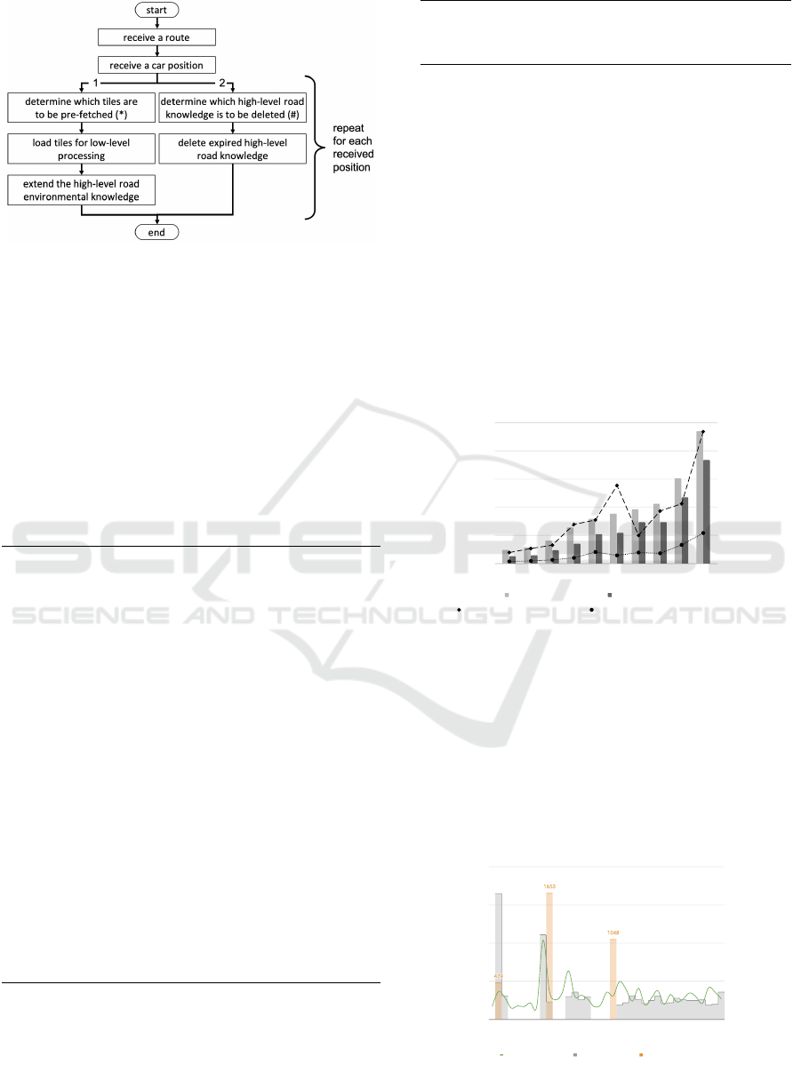
Figure 7: The method for updating the road environment

along a route with two parallel processes.

workﬂow starts with a received route and vehicle po-

sition. Next, process 1 and process 2, are started

in parallel. Process 1 (∗) determines which tiles are

required to be pre-fetched and executes the knowl-

edge abstraction process for each tile in parallel. Pro-

cess 2 (#) determines which high-level road knowl-

edge needs to be deleted. The step marked with (∗) is

modelled as SPARQL query (see Listing 1). The step

marked with (#) in process 2 is modeled as a Datalog

rule (see Listing 2). The two parallel processes repeat

for each received vehicle position.

SELECT ? t i l e I d 2 ? t i l e I d3

WHERE {

? l a : Cu r r e n tL a n e . ? rp : h a s Lane ? l .

? rp : hasNex t ? rp12 .

? rp12 : h a s Next ? rp2 2 .

? rp22 : l e n g t h ? l e n g th2 .

? rp12 : i sL o c a te d I n ? tileId2 .

? rp22 : i sL o c a te d I n ? tileId3 .

? c u rre L o c t : rem D i s O fR P ? r e ma i n in g D i s .

{ SELECT ? rp2 2 (SUM(? l e n 1 ) AS ? tL e n 1 )

WHERE {

? lane a : C u r r en t L a ne .

? rp : hasLan e ? lane .

? rp : hasNex t ? rp 1 .

? rp1 : h a s N e x t ? r p22 .

? rp1 : l e n g t h ? len1 .

}

GROUP BY ? r p 2 2

}

BIND( (? l e n g t h 2 + ? tLen1 ) AS ? t L e n 2 )

BIND( (? r e ma i n i n g D i s +? t L e n 2 ) AS ? d i s 2 )

: s pa t i a l W i n do w : f o r w ar d P ar a m e t e r ? v al .

FILTER(? d i s 2 < ? val )

}

Listing 1: A SPARQL query for pre-fetching map data tiles.

ExpiredRoadPart(r) ←

SpatialWindow(s),

NOT EXISTS r IN (RoadPart(r), inside(r, s))

Listing 2: A Datalog rule for inferring expired road parts.

4.2 Performance

We have implemented the proposed knowledge-

spatial architecture into an application called

SmartMapApp using RDFox 3.0.1 with the provided

Java APIs. The used map data covers 63.75 km

and

is split into 10 data sets for testing. The evaluation

was performed on a 64-bit Ubuntu virtual machine

with 8 Intel(R) Core(TM) i7-8550U CPU @ 1.80GHz

running at 33MHz with 15 GB memory. We recorded

the computation time after doing a warm-up run by

executing the tasks 3 times sequentially. The results

are shown in Figures 8 and 9.

Time (ms)

Number of Triple (10E2)

500

1000

1500

2000

2500

5000

7500

10000

1 2 3 4 5 6 7 8 9 10

# low-level triples # high-level triples

low2high process time extending high-level view time

Figure 8: Performance evaluation of the knowledge abstrac-

tion process.

Figure 8 illustrates the knowledge abstraction pro-

cess. The ﬁgure shows, for each data set, the number

of low-level triples (grey bar), the resulting number

of high-level triples (black bar), the time for transfer-

ring triples from the low-level to the high-level ontol-

ogy (low2high process time, diamonds), and the time

for extending the high-level road environmental view

(dot).

position

Execution & Deletion Time (ms)

Pre-lad Time (ms)

100

150

200

500

1000

1500

2000

execution time deletion time pre-loading Time

Figure 9: Performance evaluation of the spatial reasoning

process.

Ontology-based Processing of Dynamic Maps in Automated Driving

105

Figure 9 shows an excerpt of a simulation result

along a trace. The left vertical axis shows the exe-

cution and deletion time. The execution time (line)

is under 50 ms on average. The deletion time (grey

area) is almost as low as the execution time. The right

vertical axis shows the time for the pre-loading pro-

cess (orange bar). At position 18, there is a peak of

the execution time, which is 104 ms. Additionally,

the deletion time (111 ms) and the subsequent pre-

loading time (1653 ms) are both long. This indicates

that the amount of loaded data has an impact on the

execution time.

Overall, the results demonstrate the feasibility of

our ontology-based approach to process maps dynam-

ically for autonomous vehicles. The cost of reasoning

generally depends not only on the number of rules,

but also on the complexity of the combination of cer-

tain rules and the input data. For details of how RD-

Fox performs reasoning, we refer interested readers

to the description of the RDFox materialization algo-

rithm (Motik et al., 2015).

5 DISCUSSION

Existing work has shown that Datalog can be trans-

lated to SPARQL, and vice versa (Polleres, 2007;

Maier et al., 2018) and that it is feasible to use ei-

ther SPARQL or Datalog for reasoning over streams

(Rinne and Nuutila, 2017; Margara et al., 2018). The

choice of modeling rules as Datalog or SPARQL is

a trade-off between semantic expressibility and com-

putation performance. In particular, it is beneﬁcial

to study the evaluation mechanisms of Datalog (ma-

terialization) and SPARQL (graph pattern matching).

Having the advantages of each language in mind pro-

vides a practical guideline to modelling the knowl-

edge.

In our work, the datastores for the low-level on-

tologies need to perform the knowledge abstraction

process by means of primitive, transfer, distance and

bounding rules (see Section 3.2) without the necessity

to store the facts and inferred knowledge. Based on

our experiments, SPARQL queries outperform Data-

log rules considering the same desired ADAS func-

tions. Hence, all the rules in the low-level datastores

are modelled using SPARQL. However, the high-level

datastore needs to store the knowledge and perform

incremental updates by means of spatial reasoning.

This naturally leads to the modelling of the knowl-

edge as Datalog rules, taking advantage of incremen-

tal reasoning with Negation as Failure as supported

by RDFox.

6 CONCLUSIONS

In this paper, we present a a novel knowledge-spatial

architecture considering the knowledge and spatial di-

mension of map data streams. We discuss the pro-

cess of knowledge abstraction using two-level ontolo-

gies. We present the mechanism of spatial reasoning

for building a dynamic map using a spatial-window

concept. In particular, we describe how to utilize dif-

ferent types of rules to achieve two dimensional rea-

soning. We evaluated our SmartMapApp prototype

through a running example of providing a dynamic

map along a route using RDFox. We chose RDFox as

it is the only triple store that can deal with incremen-

tal reasoning with Negation as Failure. The results

of this paper demonstrate the feasibility of adopting

an ontology-based approach for processing map data

in autonomous vehicles by using a sophisticated rea-

soner with the desired scalability, such as RDFox.

In the future, we plan to extend the architecture

to ensure map data quality as there might be errors in

the raw map data. Expired road objects may also re-

sult in missing triples, where a future query might ask

for deleted objects. There needs to be a mechanism

to cache the expired road objects in order to provide

answers to such queries.

REFERENCES

Abiteboul, S., Hull, R., and Vianu, V. (1995). Foundations

of databases, volume 8.

Armand, A., Ibanez-Guzman, J., and Zinoune, C. (2017).

Digital Maps for Driving Assistance Systems and Au-

tonomous Driving, pages 201–244.

Bagschik, G., Menzel, T., and Maurer, M. (2018). Ontol-

ogy based scene creation for the development of auto-

mated vehicles. In IEEE Intelligent Vehicles Sympo-

sium (IV), pages 1813–1820.

Belouaer, L., Bouzid, M., and Mouaddib, A. (2010). Ontol-

ogy based spatial planning for human-robot interac-

tion. In 17th Int. Symposium on Temporal Represen-

tation and Reasoning (TIME 2010), pages 103–110,

Los Alamitos, CA, USA. IEEE Computer Society.

Chen, W. and Kloul, L. (2018). An ontology-based ap-

proach to generate the advanced driver assistance use

cases of highway trafﬁc. In KEOD, pages 73–81.

Cyganiak, R., Wood, D., and Lanthaler, M. (2014). RDF

1.1 Concepts and Abstract Syntax. (Accessed on

09/14/2020).

Gayathri, R. and V., U. (2018). Ontology based knowledge

representation technique, domain modeling languages

and planners for robotic path planning: A survey. ICT

Express, 4(2):69 – 74.

Gran, C. W. (2019). Hd-maps in autonomous driving. Mas-

ter’s thesis, NTNU.

KEOD 2020 - 12th International Conference on Knowledge Engineering and Ontology Development

106

Gruyer, D., Belaroussi, R., and Revilloud, M. (2016). Ac-

curate lateral positioning from map data and road

marking detection. Expert Systems with Applications,

43:1–8.

Gwon, G., Hur, W., Kim, S., and Seo, S. (2017). Genera-

tion of a precise and efﬁcient lane-level road map for

intelligent vehicle systems. IEEE Transactions on Ve-

hicular Technology, 66(6):4517–4533.

Herrtwich, R. (2018). The evolution of the HERE HD Live

Map at Daimler. (Accessed on 04/29/2020).

Hitzler, P., Krötzsch, M., Parsia, B., Patel-Schneider, P. F.,

and Rudolph, S. (27 Oct 2009). OWL 2 Web Ontology

Language: Primer (2nd Edition).

Hogan, A. (2015). Skolemising blank nodes while preserv-

ing isomorphism. In Proc. of the 24th Int. Conf. on

World Wide Web, WWW ’15, page 430–440, Repub-

lic and Canton of Geneva, CHE.

Hudelot, C., Atif, J., and Bloch, I. (2008). Fuzzy spatial

relation ontology for image interpretation. Fuzzy Sets

and Systems, 159(15):1929 – 1951. From Knowledge

Representation to Information Processing and Man-

agement.

ISO/TC 204 (2018). Intelligent transport systems-Local dy-

namic map. (Accessed on 05/27/2020).

Katsumi, M. and Fox, M. (2018). Ontologies for transporta-

tion research: A survey. Transportation Research Part

C: Emerging Technologies, 89:53 – 82.

Leite, J. (2018). A brief history of gps in-car navigation.

Liu, R., Wang, J., and Zhang, B. (2020). High deﬁnition

map for automated driving: Overview and analysis. J.

of Navigation, 73(2):324–341.

Maier, D., Tekle, K. T., Kifer, M., and Warren, D. S. (2018).

Datalog: concepts, history, and outlook. In Declara-

tive Logic Programming: Theory, Systems, and Appli-

cations, pages 3–100. ACM Books.

Margara, A., Cugola, G., Collavini, D., and Dell’Aglio, D.

(2018). Efﬁcient temporal reasoning on streams of

events with dotr. In European Semantic Web Conf.,

pages 384–399.

Mokbel, M. F., Xiong, X., Hammad, M. A., and Aref,

W. G. (2005). Continuous query processing of spatio-

temporal data streams in place. GeoInformatica,

9(4):343–365.

Motik, B., Nenov, Y., Piro, R., and Horrocks, I. (2015).

Combining rewriting and incremental materialisation

maintenance for datalog programs with equality. In

Twenty-Fourth Int. Joint Conf. on Artiﬁcial Intelli-

gence.

NDS Association (2018). The standard for map data - NDS

Association. (Accessed on 05/27/2020).

Oxford Semantic Technologies (2019). RDFox knowledge

graph system.

Polleres, A. (2007). From sparql to rules (and back).

In Proc. of the 16th Int. Conf. on World Wide Web,

WWW ’07, page 787–796, New York, NY, USA.

Qiu, H., Ayara, A., and Glimm, B. (2020). A knowledge ar-

chitecture layer for map data in autonomous vehicles.

In 2020 23rd Int. Conf. on Intelligent Transportation

Systems (ITSC). IEEE.

Rinne, M. and Nuutila, E. (2017). User-Conﬁgurable Se-

mantic Data Stream Reasoning Using SPARQL Up-

date. J. on Data Semantics, 6(3):125–138.

Shaw, M., Detwiler, L. T., Noy, N., Brinkley, J., and Su-

ciu, D. (2011). vsparql: A view deﬁnition language

for the semantic web. J. of Biomedical Informatics,

44(1):102–117.

Studer, R., Benjamins, V. R., and Fensel, D. (1998). Knowl-

edge engineering: Principles and methods. Data &

Knowledge Engineering, 25(1-2):161–197.

Suryawanshi, Y., Qiu, H., Ayara, A., and Glimm, B. (2019).

An ontological model for map data in automotive sys-

tems. In IEEE Int. Conf. on Artiﬁcial Intelligence and

Knowledge Engineering (AIKE), pages 140–147.

Ulbrich, S., Reschka, A., Rieken, J., Ernst, S., Bagschik,

G., Dierkes, F., Nolte, M., and Maurer, M. (2017). To-

wards a functional system architecture for automated

vehicles. arXiv preprint arXiv:1703.08557.

W3C SPARQL Working Group (21 Mar 2013). SPARQL

1.1 Overview.

Wache, H., Voegele, T., Visser, U., Stuckenschmidt, H.,

Schuster, G., Neumann, H., and Hübner, S. (2001).

Ontology-based integration of information-a survey of

existing approaches.

Zhao, L., Ichise, R., Liu, Z., Mita, S., and Sasaki,

Y. (2017). Ontology-based driving decision mak-

ing: A feasibility study at uncontrolled intersec-

tions. IEICE Transactions on Information and Sys-

tems, E100.D(7):1425–1439.

Ontology-based Processing of Dynamic Maps in Automated Driving

107