A Diffusion Dimensionality Reduction Approach to Background
Subtraction in Video Sequences
Dina Dushnik
1
, Alon Schclar
2
, Amir Averbuch
1
and Raid Saabni
2,3
1
School of Computer Science, Tel Aviv University, POB 39040, Tel Aviv 69978, Israel
2
School of Computer Science, The Academic College of Tel-Aviv Yaffo, POB 8401, Tel Aviv 61083, Israel
3
Triangle R&D Center, Kafr Qarea, Israel
Keywords:
Background Subtraction, Diffusion Bases, Dimensionality Reduction.
Abstract:
Identifying moving objects in a video sequence is a fundamental and critical task in many computer-vision
applications. A common approach performs background subtraction, which identifies moving objects as
the portion of a video frame that differs significantly from a background model. An effective background
subtraction algorithm has to be robust to changes in the background and it should avoid detecting non-
stationary background objects such as moving leaves, rain, snow, and shadows. In addition, the internal
background model should quickly respond to changes in background such as objects that stop or start moving.
We present a new algorithm for background subtraction in video sequences which are captured by a stationary
camera. Our approach processes the video sequence as a 3D cube where time forms the third axis. The
background is identified by first applying the Diffusion Bases (DB) dimensionality reduction algorithm to the
time axis and then by applying an iterative method to extract the background.
1 INTRODUCTION
Automatic identification of people, objects, or events
of interest are common tasks that can be found
in video surveillance systems, tracking systems,
games, etc. Typically, these systems are equipped
with stationary cameras, that are directed at offices,
parking lots, playgrounds, fences together with
computer systems that process the video data. Human
operators or other processing elements are notified
about salient events. In addition to the obvious
security applications, video surveillance technology
has been proposed to measure traffic flow, compile
consumer demographics in shopping malls and
amusement parks, and count endangered species to
name a few.
Usually, the events of interest are part of the
foreground of the video sequence and therefore
background subtraction is in many cases a
preliminary step that is applied to facilitate the
identification of the events. The difficulty in
background subtraction is not to differentiate, but to
maintain the background model, its representation
and its associated statistics. In particular, capturing
the background in frames where the background can
change over time. These changes can be moving
trees, rain, snow, sprinklers, fountains, video screens
(billboards), to name a few. Other forms of changes
are weather changes like rain and snow, illumination
changes like turning on and off the light in a room
and changes in daylight. We refer to this background
type as dynamic background while a background that
has slight or no changes at all is referred to as static
background. In this paper, we present a new method
that falls into the latter category. The main steps of
the algorithm are:
• Identification of the background by applying the
DB algorithm (Schclar and Averbuch, 2015).
• Subtract the background from the input sequence.
• Threshold the subtracted sequence.
• Detect the foreground objects by applying depth
first search (DFS).
The rest of this paper is organized as follows:
In section 2, related algorithms for background
subtraction are presented. In section 3, we
describe the DB algorithm. The proposed algorithm
is described in section 4. In section 5, we
present preliminary results that were obtained by the
proposed algorithms. We conclude in Section 6 and
provide future research options.
294
Dushnik, D., Schclar, A., Averbuch, A. and Saabni, R.
A Diffusion Dimensionality Reduction Approach to Background Subtraction in Video Sequences.
DOI: 10.5220/0010125702940300
In Proceedings of the 12th International Joint Conference on Computational Intelligence (IJCCI 2020), pages 294-300
ISBN: 978-989-758-475-6
Copyright
c
 2020 by SCITEPRESS – Science and Technology Publications, Lda. All rights reserved

2 RELATED WORK
Background subtraction is a widely used approach for
detection of moving objects in video sequences. This
approach detects moving objects by differentiating
between the current frame and a reference frame,
often called the background frame, or background
model. The background frame should not contain
moving objects. In addition, it must be regularly
updated in order to adapt to varying conditions
such as illumination and geometry changes. This
section provides a review of some state-of-the-art
background subtraction techniques. These techniques
range from simple approaches, aiming to maximize
speed and minimizing the memory requirements, to
more sophisticated approaches, aiming to achieve
the highest possible accuracy under any possible
circumstances. The goal of these approaches is to
run in real-time. We focus on methods that share
the resemble the proposed algorithm in space and
time complexity, however, additional references can
be found in (Collins et al., 2000; Piccardi, 2004;
Macivor, 2000; Bouwmans, 2014; Bouwmans et al.,
2017).
Lo and Velastin (Lo and Velastin, 2001) proposed
to use the median value of the last n frames
as the background model. This provides an
adequate background model even if the n frames are
subsampled with respect to the original frame rate
by a factor of ten (Cucchiara et al., 2003). The
median filter is computed on a special set of values
that contains the last n subsampled frames and the last
computed median value. This combination increases
the stability of the background model.
In (Wren et al., 1997) an individual background
model is constructed at each pixel location (i, j) by
fitting a Gaussian probability density function (pdf)
to the last n pixels. These models are updated via
running average given each new frame that arrives.
This method has a very low memory requirement.
In order to cope with rapid changes in the
background, a multi-valued background model was
suggested in (Stauffer and Grimson, 1999). In this
model, the probability of observing a certain pixel x
at time t is represented by a mixture of k Gaussians
distributions. Each of the k Gaussian distributions
describe only one of the observable background or
foreground objects.
A Kernel Density Estimation (KDE) of the buffer
of the last n background values is used in (Elgammal
et al., 2000). The KDE guarantees a smooth,
continuous version of the histogram of the most recent
values that are classified as background values. This
histogram is used to approximate the background pdf.
Mean-shift vector techniques have proved to be
an effective tool for solving a variety of pattern
recognition problems e.g. tracking and segmentation
((Comaniciu, 2003)). One of the main advantages
of these techniques is their ability to directly detect
the main modes of the pdf while making very few
assumptions. Unfortunately, the computational cost
of this approach is very high. As such, it cannot
be applied in a straightforward manner to model
background pdfs at the pixel level, however, in
(Piccardi and Jan, 2004; Han et al., 2004) this is
mitigated by using optimization.
Seki et al. (Seki et al., 2003) use spatial co-
occurrences of image variations. They assume that
neighboring blocks of pixels that belong to the
background should have similar variations over time.
This method divides each frame to distinct blocks
of N × N pixels where each block is regarded as an
N
2
-component vector. This trades-off resolution with
high speed and better stability. During the learning
phase, a certain number of samples is acquired at a
set of points, for each block. The temporal average
is computed and the differences between the samples
and the average, called the image variations, are
calculated. Then the N
2
× N
2
covariance matrix is
computed with respect to the average. An eigenvector
transformation is applied to reduce the dimensions of
the image variations.
This approach is based on an eigen decomposition
of the whole image (Oliver et al., 2000). During a
learning phase, samples of n images are acquired. The
average image is then computed and subtracted from
all the images. The covariance matrix is computed
and the best eigenvectors are stored in an eigenvector
matrix. For each frame I, a classification phase is
executed: I is projected onto the eigenspace and then
projected back onto the image space. The output is
the background frame, which does not contain any
small moving objects. A threshold is applied to the
difference between I and the background frame.
3 THE DB ALGORITHM
Dimensionality reduction techniques represent high-
dimensional datasets using a small number features
while preserving the information that is conveyed
by the original data. This information is mostly
inherent in the geometrical structure of the dataset.
Therefore, most dimensionality reduction methods
embed the original dataset in a low dimensional space
with minimal distortion to the original structure.
Classic dimensionality reduction techniques such as
Principal Component Analysis (PCA) and Classical
A Diffusion Dimensionality Reduction Approach to Background Subtraction in Video Sequences
295

Multidimensional Scaling (MDS) are simple to
implement and can be efficiently computed. However,
they guarantee to discover the true structure of a
data set only when the data set lies on or near a
linear manifold of the high-dimensional input space
((Mardia et al., 1979)). These methods are highly
sensitive to noise and outliers since they take into
account the distances between all pairs of points.
Furthermore, PCA and MDS fail to detect non-linear
structures.
A different and more effective dimensionality
reduction approach considers for each point only
the distances to its closest neighboring points in
the data set. These so called local methods
successfully embed the high dimensional data into an
Euclidean space of substantially smaller dimension
while preserving the geometry of the data set even
when the data set lies in a non-linear manifold. The
global geometry is preserved by maintaining the local
neighborhood geometry of each point in the data
set. Dimensionality reduction methods that employ
this approach include Local Linear Embedding (LLE)
(Roweis and Saul, 2000), ISOMAP (Tenenbaum
et al., 2000), Laplacian Eigenmaps(Belkin and
Niyogi, 2003) and Hessian Eigenmaps (Donoho and
Grimes, 2003), to name a few. Another algorithm that
falls into this category is Diffusion Maps (Coifman
and Lafon, 2006; Schclar, 2008). Diffusion Maps
preserves the random walk distance in the high
dimensional space. This distance is more robust to
noise since it averages all the paths between a pair of
points.
The Diffusion Bases (Schclar and Averbuch,
2015) dimensionality algorithm is dual to the
Diffusion Maps (Coifman and Lafon, 2006; Schclar,
2008) algorithm in the sense that it explores the
non-linear variability among the coordinates of the
original data. Both algorithms share a graph
Laplacian construction, however, the Diffusion Bases
algorithm uses the Laplacian eigenvectors as an
orthonormal system on which it projects the original
data. The Diffusion Bases algorithm has been
successfully applied for the segmentation of hyper-
spectral images (Schclar and Averbuch, 2017b;
Schclar and Averbuch, 2017a) as well as for the
detection of anomalies and sub-pixel segments in
hyper-spectral images (Schclar and Averbuch, 2019)
and is described in the following.
Let Ω =
{
x
i
}
m
i=1
, x
i
∈ R
n
, be a data set and let
x
i
( j) denote the j
th
coordinate of x
i
, 1 ≤ j ≤ n.
We define the vector y
j
= (x
1
( j) , . . . , x
m
( j)) as the
vector whose components are composed of the j
th
coordinate of all the points in Ω. The Diffusion Bases
algorithm consists of the following steps:
• Construct the data set Ω
0
=

y
j

n
j=1
• Build a non-directed graph G whose vertices
correspond to Ω
0
with a non-negative and fast-
decaying weight function w
ε
that corresponds to
the local point-wise similarity between the points
in Ω
0
. By fast decay we mean that given a
scale parameter ε > 0 we have w
ε
(y
i
, y
j
) → 0
when


y
i
− y
j


 ε and w
ε
(y
i
, y
j
) → 1 when


y
i
− y
j


 ε. One of the common choices for
w
ε
is
w
ε
(y
i
, y
j
) = exp −


y
i
− y
j


2
ε
!
(1)
where ε defines a notion of neighborhood by
defining a ε-neighborhood for every point y
i
.
• Construction of a random walk on the graph
G via a Markov transition matrix P. P is the
row-stochastic version of w
ε
which is derived by
dividing each row of w
ε
by its sum (P and the
graph Laplacian I − P (see (Chung, 1997)) share
the same eigenvectors).
• Perform an eigen decomposition of P to produce
the left and the right eigenvectors of P:
{
ψ
k
}
k=1,...,n
and
{
ξ
k
}
k=1,...,n
, respectively. Let
{
λ
k
}
k=1,...,n
be the eigenvalues of P where
|
λ
1
|
≥
|
λ
2
|
≥ ... ≥
|
λ
n
|
.
• The right eigenvectors of P constitute an
orthonormal basis
{
ξ
k
}
k=1,...,n
, ξ
k
∈ R
n
. These
eigenvectors capture the non-linear coordinate-
wise variability of the original data.
• Next, we use the spectral decay property of the
spectral decomposition to extract only the first η
eigenvectors H =
{
ξ
k
}
k=1,...,η
, which contain the
non-linear directions with the highest variability
of the coordinates of the original data set Ω. A
method for choosing η is described in (Schclar
and Averbuch, 2015).
• We project the original data Ω onto the
basis H. Let Ω
H
be the set of these
projections: Ω
H
=
{
g
i
}
m
i=1
, g
i
∈ R
η
, where g
i
=
(x
i
· ξ
1
, . .. ,x
i
· ξ
η
), i = 1, . . . , m and · denotes
the inner product operator. Ω
H
contains
the coordinates of the original points in the
orthonormal system whose axes are given by
H. Alternatively, Ω
H
can be interpreted in the
following way: the coordinates of g
i
contain the
correlation between x
i
and the directions given by
the vectors in H.
FCTA 2020 - 12th International Conference on Fuzzy Computation Theory and Applications
296

4 THE STATIC BACKGROUND
SUBTRACTION ALGORITHM
USING DB (SBSDB)
The SBSDB algorithm (Schclar, 2009; Dushnik et al.,
2013) identifies the static background, subtracts it
from the video sequence and constructs a binary mask
to describe the foreground and background. The input
to the algorithm is a gray-level video sequence. The
algorithm produces a binary mask for each video
frame.
4.1 Off-line Algorithm for Capturing
Static Background
In order to capture the static background of a scene,
we reduce the dimensionality of the input sequence
by applying the DB algorithm. The input to the
algorithm consists of n frames that form a data cube.
Formally, let D
n
=
n
s
t
i, j
, i, j = 1, ...,N, t = 1, ..., n
o
be
the input data cube of n frames each of size N ×
N where s
t
i, j
is the pixel at position (i, j) in the
video frame at time t. We define the vector U
i, j
=

s
1
i, j
, ..., s
n
i, j

to be the values of the (i, j)
th
coordinate
at all the n frames in D
n
. This vector is referred to as a
hyper-pixel. Let Ω
n
=

U
i, j

, i, j = 1, ..., N be the set
of all hyper-pixels. We define F
t
= (s
t
1,1
, ..., s
t
N,N
) to
be a 1-D vector representing the video frame at time
t. We refer to F
t
as a frame-vector. Let Ω
0
n
=
{
F
t
}
n
t=1
be the set of all frame-vectors.
We apply the DB algorithm to Ω
n
to produce
Ω
H
. The output is the projection of every hyper-
pixel on the diffusion basis which embeds the original
data D
n
into the reduced space of dimension η. The
first vector of Ω
H
represents the background of the
input frames. Let bg
V
= (x
1
, . . . , x
N
2
) be this vector.
We reshape bg
V
into the matrix bg
M
= (x
i, j
), i, j =
1, ..., N. Then, we normalize the values in bg
M
to
be between 0 to 255. The normalized background is
denoted by
c
bg
M
.
4.2 On-line Algorithm for Capturing a
Static Background
In order to make the algorithm suitable for on-
line applications, the incoming video sequence is
processed by using a sliding window of size m. Thus,
the number of frames that are input to the algorithm
is m. We denote by W
i
= (s
i
, ..., s
i+m−1
) the sliding
window starting at frame i. We seek to minimize m
in order to have low memory consumption and obtain
a faster result from the algorithm while producing a
good approximation of the background. We found
empirically that the algorithm produces good results
for values of m as low as m = 5, 6 and 7. The delay of
5 to 7 frames is negligible and renders the algorithm
to be suitable for on-line applications.
Let S = (s
1
, ..., s
m
, s
m+1
, ..., s
n
) be the input video
sequence. We apply the algorithm that is described in
section 4.1 to every sliding window. The output is a
sequence of background frames
c
BG =

(
c
bg
M
)
1
, ..., (
c
bg
M
)
m
, (
c
bg
M
)
m+1
, ..., (
c
bg
M
)
n

(2)
where (
c
bg
M
)
i
is the background that corresponds to
frame s
i
. The backgrounds of the last m − 1 frames
- (
c
bg
M
)
n−m+2
to (
c
bg
M
)
n
- are equal to (
c
bg
M
)
n−m+1
.
Figure 1 describes how the sliding window is shifted.
The sliding window facilitates a faster execution
time of the DB algorithm. Specifically, the weight
function w
ε
(Eq. 1) is not recalculated for all the
frames in the sliding window. Instead, w
ε
is only
updated according to the new frame that enters the
sliding window and the one that exits the sliding
window.
4.3 The SBSDB Algorithm
The SBSDB on-line algorithm captures the
background of each sliding window according
to section 4.2. Then it subtracts the background from
the input sequence and thresholds the output to get
the background binary mask.
Let S = (s
1
..., s
n
) be the input sequence. For each
frame s
i
∈ S, i = 1, ..., n, we do the following:
• Let W
i
= (s
i
, ..., s
i+m−1
) be the sliding window
starting at frame s
i
. The on-line algorithm for
capturing the background (section 4.2) is applied
to W
i
. The output is the background frame (
c
bg
M
)
i
.
• The SBSDB algorithm subtracts (
c
bg
M
)
i
from the
original input frame by ¯s
i
= s
i
− (
c
bg
M
)
i
. Then,
each pixel in ¯s
i
that has a negative value is set to
0.
• A threshold is applied to ¯s
i
. The calculation of
the threshold is described in section 4.4. A binary
mask is constructed in which 0 is assigned to
the background pixels and 1 is assigned to the
foreground pixels.
4.4 Threshold Computation for a Gray
Scale Input
The threshold τ is used to separate between
background and foreground pixels. It is calculated in
the last step of the SBSDB algorithm. Usually, the
A Diffusion Dimensionality Reduction Approach to Background Subtraction in Video Sequences
297

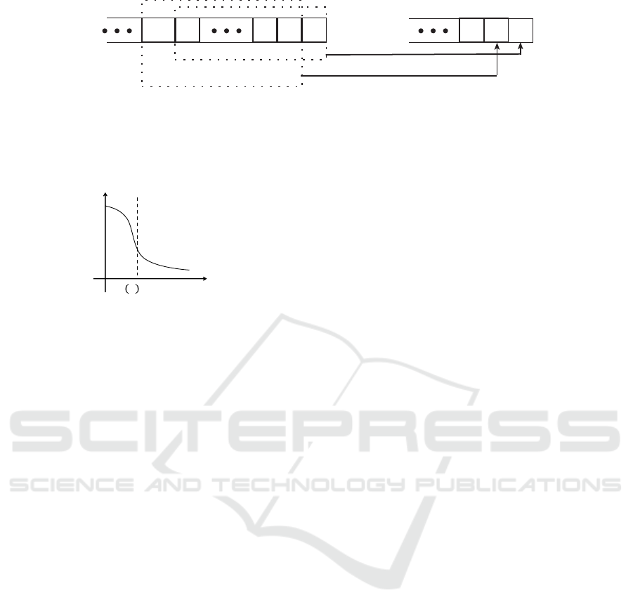
s1s2s3sm
s(m+1)
W1 size m
W2 size m
DB output for W1
DB output for W2
bg
M
^
( )
1
bg
M
^
( )
2
Figure 1: Illustration of how the sliding window is shifted. W
1
= (s
1
, ..., s
m
) is the sliding window for s
1
. W
2
= (s
2
, ..., s
m+1
)
is the sliding window for s
2
, etc. The backgrounds of s
i
and s
i+1
are denoted by (
c
bg
M
)
i
and (
c
bg
M
)
i+1
, i = 1, ..., n − m + 1,
respectively.
𝜏
𝒉
′
𝒙 > 𝝁, 𝝁 < 𝟎
Figure 2: An example how to find the threshold value τ in a
given histogram h. τ is set to x since at x we have h
0
(x) < µ.
histogram of a frame after subtraction will be high
at small values and low at high values. The SBSDB
algorithm smooths the histogram in order to compute
the threshold value accurately.
Let h be the histogram of a frame and let µ < 0
be a given parameter which provides a threshold for
the slope of h. µ is chosen to be the magnitude of
the slope where h becomes moderate. We scan h
from its global maximum to the minimum. We set the
threshold τ to the smallest value x that satisfies h
0
(x) >
µ where h
0
(x) is the first derivative of h at point x, i.e.
the slope of h at point x. The background/foreground
classification of the pixels in the input frame ¯s
i
is
determined according to τ. Specifically, a binary
mask
e
s
i
is constructed as follows:
˜s
i
(k, l) =

0
1
i f ¯s
i
(k, l) < τ
otherwise
k, l = 1, ..., N
Fig. 2 illustrates how to find the threshold.
The SBSDB algorithm can be executed in
parallel in a very simple manner. First, the
data cube D
n
=
n
s
t
i, j
, i, j = 1, ..., N, t = 1, ..., n
o
is decomposed into c × d overlapping data
cubes

β
k,l

k=1,...c,l=1,...d
where β
k,l
=
n
s
t
i, j
,
i = i
k
, ..., (i
k+1
− 1), j = j
l
, ..., (i
l+1
− 1), t = 1, ..., n
}
.
Next, the SBSDB algorithm is applied to each
individual block. This step can run in parallel.
The final result of the algorithm is constructed by
placing each block at its original location in D
n
. The
result for pixels that lie in overlapping areas between
adjacent blocks is obtained by applying a logical OR
operation to the corresponding blocks results.
5 EXPERIMENTAL RESULTS
We apply the SBSDB algorithm to an AVI video
sequence that consists of 190 gray scale frames of
size 256 × 256. The video sequence was captured
by a stationary camera and its frame rate is 15 fps.
The video sequence shows moving cars over a static
background. We apply the sequential version of the
algorithm where the size of the sliding window is
set to 5 and reduced the dimensionality to 1. We
also apply the parallel version of the algorithm where
the video sequence is divided to four blocks in a
2 × 2 formation. The overlapping size between two
(either horizontally or vertically) adjacent blocks is
set to 20 pixels and the size of the sliding window is
set to 10. The values of the parameters were found
empirically. Let s be a test frame and let W
s
be the
sliding window starting at s. In Fig. 3 we show the
frames that W
s
contains. The output of the SBSDB
algorithm for s is shown in Fig. 4. The background is
subtracted accurately and the moving cars are clearly
classified as the foreground. Moreover, the algorithm
successfully detects small foreground objects such as
the moving arms of the pedestrian that is walking on
the left sidewalk.
6 CONCLUSION AND FUTURE
WORK
We introduced in this work an algorithm for automatic
background subtraction of video sequences with static
background. The algorithm captures the background
by reducing the dimensionality of the input via the
Diffusion Bases algorithm. The SBSDB algorithm
can be applied on-line. The algorithm accurately
models the background of the input video sequences.
The performance of the proposed algorithm can
be enhanced by improving the accuracy of the
threshold values. Furthermore, it is necessary
to develop a data-driven method for automatic
computation of µ, which is used in the threshold
FCTA 2020 - 12th International Conference on Fuzzy Computation Theory and Applications
298

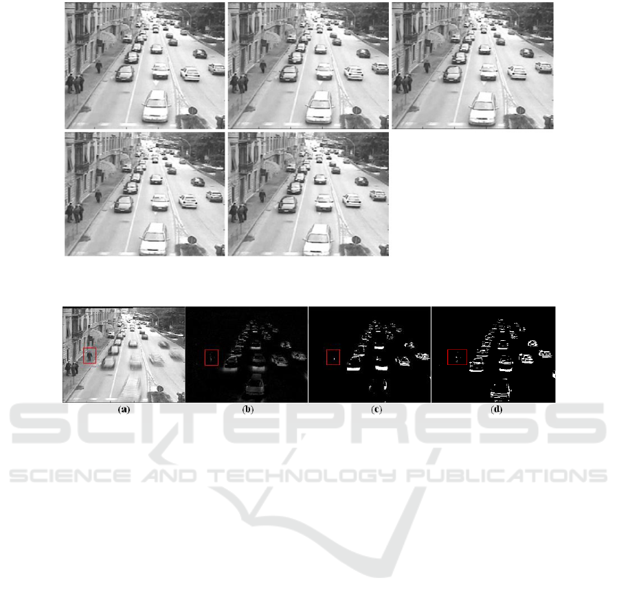
Figure 3: The frames that W
s
contains. The test frame s is at the top-left corner. The frames are ordered from top-left to
bottom-right.
Figure 4: Results of the SBSDB algorithm when allpied to the sliding window in Fig. 3. (a) The background for the test frame
s. (b) The test frame s after the subtraction of the background. (c) The binary mask output of the sequential algorithm for the
test frame s. (d) The binary mask output for the test frame s from the parallel version of the algorithm.
computation (sections 4.4). Additionally, the
proposed algorithms can be useful to achieve low-
bit rate video compression for transmission of rich
multimedia content. The captured background
can be transmitted once followed by the detected
segmented objects. Furthermore, the authors are in
the final stages of extending the proposed algorithm
to handle video sequences that contain non-static
background. Lastly, another extension that is
currently being developed to handle video sequences
that are captured by non-stationary cameras. This
application is becoming more and more important
given the increasing utilization of drones.
REFERENCES
Belkin, M. and Niyogi, P. (2003). Laplacian eigenmaps
for dimensionality reduction and data representation.
Neural Computation, 15(6):1373–1396.
Bouwmans, T. (2014). Traditional and recent approaches
in background modeling for foreground detection: An
overview. Computer Science Review, 11-12:31–66.
Bouwmans, T., Maddalena, L., and Petrosino, A. (2017).
Scene background initialization: A taxonomy. Pattern
Recognition Letters, 96:3–11. Scene Background
Modeling and Initialization.
Chung, F. R. K. (1997). Spectral Graph Theory. AMS
Regional Conference Series in Mathematics, 92.
Coifman, R. R. and Lafon, S. (2006). Diffusion maps.
Applied and Computational Harmonic Analysis,
21:5–30.
Collins, R., Lipton, A., and Kanade, T. (2000). Introduction
to the special section on video surveillance. IEEE
Transactions on Pattern Analysis and Machine
Intelligence, 22(8):745–746.
Comaniciu, D. (2003). An algorithm for data-driven
bandwidth selection. IEEE Transactions on Pattern
Analysis and Machine Intelligence, 25(2):281–288.
Cucchiara, R., Grana, C., Piccardi, M., and Prati, A. (2003).
Detecting moving objects, ghosts, and shadows in
video streams. IEEE Transactions on Pattern Analysis
and Machine Intelligence, 25(10):1337–1442.
Donoho, D. L. and Grimes, C. (2003). Hessian eigenmaps:
new locally linear embedding techniques for high-
dimensional data. In Proceedings of the National
Academy of Sciences, volume 100, pages 5591–5596.
Dushnik, D., Schclar, A., and Averbuch, A. (2013).
Video segmentation via diffusion bases. CoRR,
http://arxiv.org/abs/1305.0218.
A Diffusion Dimensionality Reduction Approach to Background Subtraction in Video Sequences
299

Elgammal, A., Hanvood, D., and Davis, L. S. (2000).
Nonparametric model for background subtraction.
Proceedings of the European Conference on
Computer Vision, pages 751–767.
Han, B., Comaniciu, D., and Davis, L. S. (2004).
Sequential kernel density approximation through
mode propagation: applications to background
modeling. Proceedings of the Asian Conference on
Computer Vision.
Lo, B. P. L. and Velastin, S. A. (2001). Automatic
congestion detection system for underground
platforms. Proc. ISIMP, pages 158–161.
Macivor, A. M. (2000). Background subtraction techniques.
Proc. of Image and Vision Computing.
Mardia, K. V., Kent, J. T., and Bibby, J. M. (1979).
Multivariate Analysis. Academic Press, London.
Oliver, N. M., Rosario, B., and Pentland, A. P. (2000). A
bayesian computer vision system for modeling human
interactions. IEEE Transactions on Pattern Analysis
and Machine Intelligence, 22(8):831–843.
Piccardi, M. (2004). Background subtraction techniques:
a review. IEEE International Confrence on Systems,
Man and Cybernetics.
Piccardi, M. and Jan, T. (2004). Efficient mean-shift
backgonmd subtraction. Proc. of IEEE KIP.
Roweis, S. T. and Saul, L. K. (2000). Nonlinear
dimensionality reduction by locally linear embedding.
Science, 290:2323–2326.
Schclar, A. (2008). A Diffusion Framework for
Dimensionality Reduction, pages 315–325. Springer
US, Boston, MA.
Schclar, A. (2009). Multi-sensor fusion via
reduction of dimensionality. PhD thesis,
https://arxiv.org/pdf/1211.2863.pdf.
Schclar, A. and Averbuch, A. (2015). Diffusion bases
dimensionality reduction. In Proceedings of the
7th International Joint Conference on Computational
Intelligence (IJCCI 2015) - Volume 3: NCTA, Lisbon,
Portugal, November 12-14, 2015., pages 151–156.
Schclar, A. and Averbuch, A. (2017a). A diffusion
approach to unsupervised segmentation of hyper-
spectral images. In Computational Intelligence - 9th
International Joint Conference, IJCCI 2017 Funchal-
Madeira, Portugal, November 1-3, 2017 Revised
Selected Papers, pages 163–178.
Schclar, A. and Averbuch, A. (2017b). Unsupervised
segmentation of hyper-spectral images via diffusion
bases. In Proceedings of the 9th International Joint
Conference on Computational Intelligence, IJCCI
2017, Funchal, Madeira, Portugal, November 1-3,
2017., pages 305–312.
Schclar, A. and Averbuch, A. (2019). Unsupervised
detection of sub-pixel objects in hyper-spectral images
via diffusion bases. In Proceedings of the 11th
International Joint Conference on Computational
Intelligence, IJCCI 2019, Vienna, Austria, September
17-19, 2019., pages 496–501.
Seki, M., Wada, T., Fujiwara, H., and Sumi, K. (2003).
Background subtraction based on cooccurrence of
image variations. Proceedings of the International
Conference on Computer Vision and Pattern
Recognition, 2:65–72.
Stauffer, C. and Grimson, W. E. L. (1999). Adaptive
background mixture models for real-time tracking.
IEEE Computer Vision and Pattern Recognition,
pages 246–252.
Tenenbaum, J. B., de Silva, V., and Langford, J. C.
(2000). A global geometric framework for nonlinear
dimensionality reduction. Science, 290:2319–2323.
Wren, C., Azarhayejani, A., Darrell, T., and Pentland, A. P.
(1997). Pfinder: real-time tracking of the human body.
IEEE Transactions on Pattern Analysis and Machine
Analysis, 19(7):780–785.
FCTA 2020 - 12th International Conference on Fuzzy Computation Theory and Applications
300