
Behavioral Locality in Genetic Programming
Adam Kotaro Pindur
a
and Hitoshi Iba
Department of Information and Communication Engineering, Graduate School of Information Science and Technology,
University of Tokyo, Tokyo, Japan
Keywords:
Genetic Programming, Locality, Distance Metrics, Tree Edit Distance, Graph Kernel.
Abstract:
Locality is a key concept affecting exploration and exploitation in evolutionary computation systems. Geno-
type to phenotype mapping has locality if the neighborhood is preserved under that mapping. Unfortunately,
assessment of the locality in Genetic Programming is dependent on the distance metric used to compare pro-
gram trees. Furthermore, there is no distinction between genotype and phenotype in GP. As such the definition
of locality in GP was studied only in the context of genotype-fitness mapping. In this work we propose a dif-
ferent family of similarity measures, graph kernels, as alternatives to the traditional family of distance metrics
in use, that is edit distance. Traditional tree edit distance is compared to the Weisfeiler-Lehman Subtree Ker-
nel, which is considered to be the state-of-the-art method in graph classification. Additionally, we extend the
definition of the locality of GP, by studying the relationship between genotypes and behaviors. In this paper,
we consider a mutation-based GP system applied to two basic benchmark problems: artificial ant (multimodal
deceptive landscape) and even parity (highly neutral landscape).
1 INTRODUCTION
The most important question in Evolutionary Com-
putation (EC) field is: ”How to characterize, study
and predict EC search?” Various approaches were em-
ployed to answer this question. These are Micro-
scopic Dynamical System Models, Component Anal-
ysis, Schema Theories, and Fitness Landscape.
Fitness Landscape is a metaphor used to visualize
problems and is also most commonly used to define
a problem difficulty. In the simplest form, a fitness
landscape can be represented as a two-dimensional
plot of an individual against its fitness. Furthermore,
if the genotype can be visualized in two dimensions,
the plot can be seen as a three-dimensional map with
peaks, valleys, hills, and plateaus. This representation
of a search space incorporates the concept of neigh-
bors (Langdon and Poli, 2013). To properly under-
stand the features of the landscape and exploit it, we
need to understand how a neighborhood of a point
looks like. Additionally, to understand how an evo-
lutionary algorithm explores and exploits such a land-
scape, it is necessary to understand the locality of rep-
resentations and operators used during the evolution-
ary process.
In an abstract sense, the locality of an operator (of
a
https://orcid.org/0000-0002-7980-265X
a mapping) refers to how well such an operator pre-
serves the neighborhood of a point. In the context of
evolutionary algorithms, small changes in genotype
space should correspond to small changes in pheno-
type space. The most extensive work on the topic of
locality in EC has been presented in (Rothlauf, 2006),
which has analyzed the importance of locality in per-
forming an effective search over a given landscape.
However, studies on locality in tree-based GP are still
very rare (Poli et al., 2008). A study of genotype
to fitness mapping was proposed in (Galv
´
an-L
´
opez
et al., 2010b) as an alternative to standard genotype-
phenotype mapping, which cannot be simply used
for typical GP. That is, there is no distinction be-
tween genotypes and phenotypes in GP. However, it
is more natural to consider mapping from genotype
to some kind of phenotype, an intermediate form be-
tween genotype and its fitness.
Therefore in this work, we are interested in inves-
tigating the locality of genotype-behavior mapping.
That is, we want to study the locality present in GP for
behaviors of evolved individuals. For this purpose, we
use three basic mutation operators (subtree, structural,
and one-point (Koza, 1992)), and study their behav-
ior using two distance measures defined on tree struc-
tures. In addition to traditionally used Tree Edit Dis-
tance (TED), we also propose using a new family of
Pindur, A. and Iba, H.
Behavioral Locality in Genetic Programming.
DOI: 10.5220/0010113400810091
In Proceedings of the 12th International Joint Conference on Computational Intelligence (IJCCI 2020), pages 81-91
ISBN: 978-989-758-475-6
Copyright
c
2020 by SCITEPRESS – Science and Technology Publications, Lda. All rights reserved
81

similarity measures, referred to as Graph Kernels. Lo-
calities of these operators are studied for artificial ant
problem (with multimodal landscape (Langdon et al.,
1998)) and even parity problem (with neutral land-
scape (Galvan-Lopez, 2009)).
2 PRELIMINARIES
2.1 Locality
The locality is an essential concept in EC, which
affects how an algorithm explores and exploits the
search space. In the sense of EC, a genotype to pheno-
type mapping has locality if the neighborhood is pre-
served under that mapping. The study of locality is
important for two reasons: (i) locality can be used as
an indicator of problem difficulty; (ii) to successfully
search the space, a small change in genotype should
result in a small change of fitness.
In (Rothlauf, 2006) definition of locality assumes
that a distance measure exists on both genotype and
phenotype spaces. Additionally, it should be possi-
ble to define the neighborhood in terms of minimum
distance. There are two types of locality: low and
high. A representation is said to have a high locality
if neighboring genotypes correspond to neighboring
phenotypes. Conversely, in representation with a low
locality, neighboring genotypes do not correspond
to neighboring phenotypes. According to (Galv
´
an-
L
´
opez et al., 2010b), representations with high local-
ities are more efficient at evolutionary search. That
is, any search operator has the same effect in both the
genotype and phenotype space. In this case, the prob-
lem difficulty is unchanged.
On the other hand when the locality is low, (Jones
et al., 1995) considers three categories:
1. easy, fitness is positively correlated with the dis-
tance to the global optimum,
2. difficult, there is no correlation between fitness
and distance from the global optimum,
3. misleading, fitness is negatively correlated with
the distance to the global optimum.
If a given problem is easy, then the low locality rep-
resentation will make it harder, that is, will convert
the problem type to difficult. This is the result of the
uncorrelated fitness landscape of the low locality rep-
resentations, which randomizes the search. If a prob-
lem is difficult, then the difficulty is unchanged. In
rare cases, there are representations that can convert
a problem from difficult to easy. Finally, if the prob-
lem is of the third category, a low locality representa-
tion will convert it to a difficult problem. That is, the
problem becomes easier because the search is more
random.
In Genetic Programming, there is no distinction
between genotypes and phenotypes, therefore, the
locality in GP was studied in terms of genotype-
fitness mapping instead (Galv
´
an-L
´
opez et al., 2010a;
Galv
´
an-L
´
opez et al., 2010b).
2.2 Distance Metrics
For evolutionary algorithms with simple genotypes,
such as genetic algorithms with binary representa-
tion, distance can be evaluated using Hamming dis-
tance (Belea et al., 2004). On the other hand, when
the genotype becomes more complex, e.g. trees in
GP, then more sophisticated methods are necessary.
The most commonly used dissimilarity measures in
EC belong to the family of edit distances (Gustafson
and Vanneschi, 2008).
Another set of methods that are used in evaluating
distance between trees are various tests for isomor-
phism. In (Burke et al., 2004), they are referred to as
pseudo-isomorphisms, which were found by defining
a three-tuple of hterminals, non-terminals, depthi. Ap-
proaches, such as genetic markers (Burks and Punch,
2015) and hybrid methods (Kelly et al., 2019), belong
to this group of methods. In this setting, two trees
are the same if and only if their respective tuples are
the same. These methods are used because exact tests
for isomorphism were, and in some cases still are, too
computationally expensive.
Lastly, a new class of algorithms for graph com-
parisons have been proposed and improved over time.
These methods are referred to as graph kernels and
are widely used in fields such as chemoinformat-
ics, bioinformatics, and natural language processing
(Nikolentzos et al., 2019). While these methods were
developed for use with more complex graphs, they
can also be used for simpler structures. In this con-
text, GP syntax trees can be defined as connected
acyclic graphs, therefore, graph kernels can be used
as a distance metric.
The following subsections provide a brief intro-
duction to the topics of (i) edit distance; (ii) kernel
methods; and (iii) graph kernel methods.
2.2.1 Edit Distance
Edit distance is a family of distance metrics defined
on non-vectorial data, such as strings, trees, and
graphs. The Levenshtein distance is a well-known
edit distance method, which is used to measure the
distance between two sequences, for example, strings.
The distance between two strings is given by the min-
imum number of operations, insertion, deletion, or
ECTA 2020 - 12th International Conference on Evolutionary Computation Theory and Applications
82

substitution, required to transform one string to an-
other.
Generalization of the edit distance for more com-
plex data structures, namely trees, was introduced in
(Tai, 1979) and was later referred to as Tree Edit Dis-
tance (TED). Edit distance was introduced to the field
of EC as a distance metric in (O’Reilly, 1997), to mea-
sure the degree of dissimilarity between two tree-like
structures. More formally, let G and G
0
be two rooted
trees where each vertex is assigned a label from al-
phabet Σ. The edit distance between these two trees
is the minimum cost of transforming G into G
0
using
a sequence of operations (single operation per node):
(i) substitution of a node v, that is, change its label;
(ii) deletion of the node v and resetting the children as
the children of v’s parent; and (iii) insertion of a node
v, as a reverse of the deletion operation.
2.2.2 Graph Kernel Methods
Classical learning algorithms use instances, e.g. x, x
0
in non-empty set X , through an inner product hx, x
0
i.
This can be interpreted as a distance, or similarity be-
tween instances x and x
0
. The biggest advantage of
kernel methods is that they can operate on any type
of data. The input space X is not restricted to vector
space, and it can be applied to structured domains,
such as strings or graphs. Kernels can be used on
structured data as long as an appropriate mapping to
RKHS H can be found, that is φ : X → H . How-
ever, the structure of the graph is invariant to permu-
tations of its representations. That is, the ordering of
the nodes and edges does not change the structure of
the graph. Therefore, similarity measures also have
to take into account this property. Various paradigms
were proposed to evaluate similarity in such a way.
These methods can be roughly divided into follow-
ing subgroups: neighborhood aggregation methods,
assignment kernels, matching-based kernels, walks
and paths based kernels, and finally subgraph pattern-
based kernels (Kriege et al., 2020). The last paradigm
seems to be the most natural way to define kernel
methods on structured data. This class of functions
is based on the decomposition of the object into sub-
structures, e.g. subgraphs or vertices, which are then
compared by applying existing kernels. Such kernels
are referred to as R -convolution kernels.
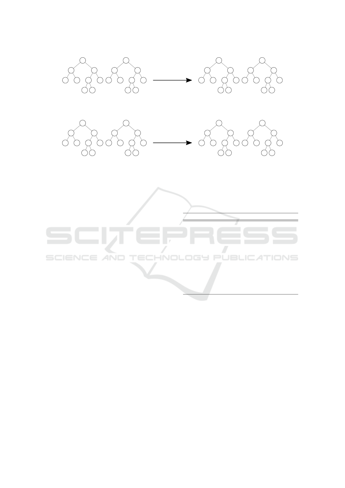
2.2.3 Weisfeiler-Lehman Framework
The Weisfeiler-Lehman algorithm/framework was in-
spired by the Weisfeiler-Lehman’s graph isomor-
phism test, also known as ”naive vertex refinement”.
This framework can be applied to any graph ker-
nel, such as the shortest path or subtree kernel (Sher-
vashidze et al., 2011). Among those, the Weisfeiler-
Lehman subtree kernel is considered to be the state-
of-the-art algorithm in graph classification. The key
idea of this algorithm is to augment labels of each
node with so-called multiset label consisting of the
original label of the vertex and sorted labels of its
neighborhood. This newly created multiset is then
compressed, resulting in a new and short label (shown
in Figure 1). Relabeling procedure is repeated for h
iterations, and two nodes from different graphs will
match if and only if they have identical multiset la-
bels. Formally, the Weisfeiler-Lehman Framework
can be defined as follows:
Definition 1. (Weisfeiler-Lehman Framework)
(Nikolentzos et al., 2019)
Let k be any kernel for graphs, that we will call
the base kernel. Then the Weisfeiler-Lehman kernel
with h iterations with the base kernel k between two
graphs G and G
0
is defined as:
k
W L
(G, G
0
) = k(G
0
, G
0
0
) + k(G
1
, G
0
1
) + ·· · + k(G
h
, G
0
h
),
(1)
where h is the number of Weisfeiler-Lehman itera-
tions, and {G
0
, G
1
, . . . , G
h
} and {G
0
0
, G
0
1
, . . . , G
0
h
} are
the Weisfeiler-Lehman sequences of G and G
0
, respec-
tively.
The above definition states, that any graph kernel
which considers graphs with discrete node labels can
take advantage of the Weisfeiler-Lehman framework.
Furthermore, if the base kernel compares subtrees of
two graphs G and G
0
, then the method is referred to
as the Weisfeiler-Lehman Subtree Kernel. For further
information (on both theory and implementation), see
(Nikolentzos et al., 2019) and (Kriege et al., 2020).
3 EXPERIMENTAL SETUP
Many studies try to improve GP, by incorporating se-
mantic information during exploration and exploita-
tion of the search space (Vanneschi et al., 2014). Un-
fortunately, most studies are purely empirical with no
theoretical backing. Most of the works are based on
experience rather than mathematics. To solve this is-
sue, a lot of work was done to understand how the
locality of both representations and genetic operators
affect the problem difficulty. This approach, while be-
ing straightforward for simple structures used in GAs,
is troublesome when applied to tree-based GP. Geno-
type to phenotype mapping cannot be simply studied,
as there is no clear distinction between representation
(genotype) and solution (phenotype). Therefore, most
works consider genotype-fitness mapping. However,
it is more natural to consider mapping from genotype
Behavioral Locality in Genetic Programming
83
+
−
x
1
5
·
+
1
x
2
2
+
−
x
1
5
+
·
1
x
2
2
G
G
0
0, 12
1,035
3,1 5,1
2,005
0,245
5,0 4,0
5,2
0,01
1,035
3,1 5,1
0,025
2,045
5,2 4,2
5,0
G
G
0
0,01 → 6 3,1 → 13
0,12 → 7 4,0 → 14
0,025 → 8 4, 2 → 15
0,245 → 9 5, 0 → 16
1,035 → 10 5, 1 → 17
2,005 → 11 5, 2 → 18
2,045 → 12
+ → 0
− → 1
· → 2
x
1
→ 3
x
2
→ 4
c → 5
0
1
3 5
2
0
1 4
5
0
1
3 5
0
2
1 4
5
G
G
0
7
10
13 17
11
9
16 14
18
6
10
13 17
8
9
18 15
16
G
G
0
Figure 1: Illustration of the relabeling process used in the Weisfeiler-Lehman subtree kernel for h = 1 for two trees G and G
0
.
In the Genetic Programming setting, node labels are first relabeled from mathematical operations into simpler representation,
e.g. integers (top). In the following step, node labels are augmented with multiset labels, which consist of the original label of
the node and sorted labels of its neighborhood (a tree with multiset labels is presented in the bottom left). Created multiset is
compressed by relabeling it with a new label, which did not exist in the original set of labels. Relabeling scheme is presented
in the bottom middle, and relabeled trees are shown in the bottom right.
to some intermediate form, such as the behavior of an
individual. In this work, we study the locality of geno-
type to behavior mapping for three basic mutation op-
erators: subtree, structural, and one-point. This is
examined for two benchmark problems: (i) Artificial
Ant; and (ii) Even-n-Parity.
Artificial Ant is often used as a GP benchmark
problem. It consists of finding a program that can
successfully navigate an artificial ant along a path
on a 32 × 32 toroidal grid. The most commonly
used trail (called Santa Fe trail) consists of 89 pel-
lets of food, and the number of pellets eaten by
an ant is its fitness. Standard set of non-terminals
F = {IfFoodAhead, prog2, prog3} and terminals T =
{Move, Right, Left} is used. In this study we con-
sider the behavior of the artificial ant to be its se-
quence of moves and positions. That is, each indi-
vidual in population is associated with a vectors of
the form (x, y, dir), where x, y are positions in space
and dir is the direction faced by an ant with val-
ues: {north, east, south, west}. Program times-out af-
ter 600 steps, thus, behavioral differences between the
individuals can be determined by simply comparing
these vectors.
The goal of the boolean Even-n-Parity problem is
to evolve a function that returns true if an even num-
ber of the inputs evaluates to true, and false other-
wise. GP uses set of terminals (n = 6 inputs), and
non-terminals F = {NOT, OR, AND}. Fitness of a
program is the number of successfull parity evalua-
tions, thus, the maximum fitness is 2
6
= 64. The be-
havior of a program can be defined in terms of the out-
Table 1: Common GP parameters.
Parameters Values
Population size 500
Initialization Ramped half and half
Max depth 6
Selection Tournament
Size 7
Generations 50
Runs 50
Crossover rate 70%
Mutation rate 30%
Max depth 2
Static tree height limit 20
puts it produces. Outputs are recorded as sequences of
binary values for each of the test cases used during fit-
ness evaluations. Behavioral differences between the
individuals can be calculated by comparing sequences
of outputs.
Parameters of the GP used to solve artificial ant
and even-6-parity problems are presented in Table 1.
Population size was set to 500 and was initialized with
ramped half and half method (Koza, 1992). The initial
population consists of trees with heights from 1 to 6.
Programs were evolved for 50 generations. Crossover
rate was set to 70% and parents were selected using
tournament selection of size 7. Additionally, individ-
uals were mutated with the probability of 30% us-
ing one of the three mutation operators: (i) subtree,
replaces a randomly selected subtree with randomly
created subtree; (ii) structural, either inflates or de-
flates the individual; or (iii) one-point, replaces a sin-
ECTA 2020 - 12th International Conference on Evolutionary Computation Theory and Applications
84

gle node in the individual. Subtree mutation was re-
stricted to generating subtrees with a maximum height
of 2. To avoid excessive bloat of the trees, a static
height limit of 20 was set for a crossover operator.
That is, if crossover operation resulted in an offspring
with a height greater than 20, then the offspring was
replaced by one of the parents at random. However,
this limit does not affect mutation operators, as they
are limited in the growth of the trees. This GP run was
repeated 50 times to collect the appropriate amount of
statistical data. A set of experiments was conducted
to examine proposed approaches.
Before proceeding with investigating the behav-
ioral locality of mutation operators, we have to deter-
mine the differences between two distance measures
used in this study.
A conventional distance measure, Tree Edit Dis-
tance considers the distance between the trees to be
the minimum amount of edits needed to transform one
tree to another. Thus, it takes into account only lo-
cal properties. This approach provides us with a fine-
grained distance (a measure of dissimilarity) between
the individuals, in the form of an integer with the
maximum distance being |G
1
| + |G
2
|, where |G
1
| and
|G
2
| are the number of nodes of compared trees G
1
and G
2
. Zhang and Shasha’s dynamic programming
implementation of TED (Zhang and Shasha, 1989)
was applied in this study.
On the other hand, the Weisfeiler-Lehman Sub-
tree Kernel is a method of evaluating the similarity
between the trees. Similarly to TED, this method re-
turns an integer value. However, this value defines the
closeness of individuals. That is, the higher the value,
the more similarities are shared between individuals.
To compare this method to TED it is necessary to con-
vert similarity value to dissimilarity by first normaliz-
ing similarity (
k(G,G
0
)
k(G,G)+k(G
0
,G
0
)
), and then subtracting it
from 1.
These methods were compared by calculating the
average dissimilarity of an individual to the rest of the
population. This is done by creating a matrix consist-
ing of pairwise distances, which is further summed
for one of the axes. A vector of values received in this
way represents the distribution of average dissimilar-
ities and is plotted against indices used to label indi-
viduals. This comparison was executed for the pop-
ulation in the last generation of GP run, which was
repeated 50 times, to examine an average difference
in behaviors of these two methods.
After the initial investigation of differences be-
tween distance measures, we proceeded with the in-
vestigation of the behavioral locality of mutation op-
erators. To have sufficient statistical data, we have
created 1, 250, 000 individuals. This was achieved by
recording all individuals created during the evolution
of GP with parameters as defined in the Table 1. All
three mutation operators were used in the evolution-
ary process, to avoid bias in data. Gathered individ-
uals were mutated using subtree, structural and one-
point mutations. Finally, data created in such a way
was divided into parts consisting of positive, neutral,
and negative mutations, that is, mutations which in-
creased, did not change, and decreased fitness of an
individual, respectively.
In the first set of results, this data was used to
present occurrences of individuals with positive, neu-
tral, and negative mutations for subtree, structural and
one-point mutations. These results are necessary to
determine what kind of distribution was created by
our experimental setup, thus, allowing us to directly
compare these results with past investigations.
The second set of results present distributions of
fitness and behavior distance with respect to the fre-
quency of such a mutation occurring. In this case, we
plotted an absolute fitness distance, as it is not impor-
tant if the change was positive or negative. We are
interested in how often fitness and behavior distance
of 1 occurred. That is, the most frequently occurring
mutation operator can be said to be of the highest lo-
cality.
Finally, this work presents fitness distance, behav-
ior distance, tree edit distance, and WL-Subtree Ker-
nel distance plotted against the fitness of an individual
before mutation (referred to as original fitness). This
subset of results is presented in the form of a 3 × 4
grid, with rows corresponding to mutation operators.
Three super-sets of results are presented for positive,
neutral, and negative mutations. Due to space restric-
tions, this result is shown only for an artificial ant
problem. This representation should allow us to see
an average structural change (in terms of TED and
WL-Subtree Kernel) introduced by mutation opera-
tors. At the same time, the use of the same x-axis
allows us to see how this structural change relates to
fitness and behavioral changes.
4 RESULTS AND DISCUSSION
A comparison between TED and WL-Subtree Kernel
is presented in Figure 2. Individuals in the popula-
tion were sorted with respect to their sizes (number
of nodes in the tree). That is, individuals on the left
side (closer to 0) consist of fewer nodes than individ-
uals to the right (closer to 500). For all tested cases,
TED (depicted with orange lines) returns higher aver-
age distances than WL-Subtree Kernel (shown as blue
lines). On the other hand, differences between those
Behavioral Locality in Genetic Programming
85
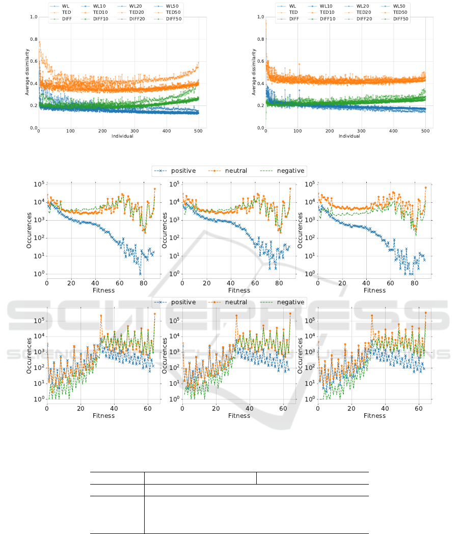
Figure 2: Distribution of average dissimilarity vs label of an individual for artificial ant (left) and even-6-parity (right).
Figure 3: Occurrences of individuals after applying subtree (left), structural (middle), and one-point mutation (right). Results
for artificial ant problem (top) and even-6-parity (bottom).
Table 2: Frequencies of subtree, structural and one-point mutations leading to fitness and behavior distance to be 1.
Artificial Ant Even-6-Parity
Fitness Behavior Fitness Behavior
Subtree 2.86 · 10
−2
6.17 · 10
−5
1.75 · 10
−2
9.06 · 10
−3
Structural 2.96 ·10
−2
4.25 · 10
−5
1.33 · 10
−2
7.10 · 10
−3
One-Point 1.65 · 10
−2
1.85 · 10
−5
1.19 · 10
−2
6.57 · 10
−3
two values are fairly stable (green line). This is the
difference in dissimilarity evaluation between TED,
which computes dissimilarity by considering only lo-
cal differences, and WL-Subtree kernel, which con-
siders both local and global properties of the trees.
WL-Subtree kernel calculates the similarity by taking
into account several feature vectors, created through
the relabeling procedure, as shown in Figure 1. As
an effect, it ”dilutes” small differences, thus consid-
ers trees to be more similar. This is more visible for
bigger individuals, where the difference between the
two methods is increasing (seen as a rise in values
presented by the green line).
Figure 3 shows the occurrences of individuals af-
ter applying three mutation operators. For artificial
ant problem, we can observe various peaks of neutral
ECTA 2020 - 12th International Conference on Evolutionary Computation Theory and Applications
86
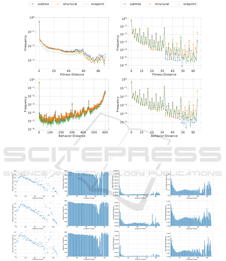
Figure 4: Distribution of fitness distance (top) and behavior distance (bottom) vs frequency. Results for the artificial ant
problem (left) and even-6-parity (right) using subtree, structural, and one-point mutation.
Figure 5: Results after applying subtree (top), structural (middle), and one-point mutation (bottom) for an artificial ant prob-
lem. Original fitness vs positive fitness (first column), original fitness vs behavior distance (second column), and structural
distance metrics using edit distance (third column) and Weisfeiler-Lehman Subtree Kernel (fourth column).
and negative mutations in the fitness range. The first
set of peaks can be observed for low fitness values
(< 15). This is consistent with results given in (Lang-
don and Poli, 2013), where it was shown that the
number of individuals with low fitnesses (regardless
of their size) is always high in artificial ant problem.
However, similarly high peaks can also be observed in
the fitness range of [50, 70]. However, these peaks ap-
pear in the distribution of fitness values in the search
space, thus are unique to the problem rather than to
Behavioral Locality in Genetic Programming
87
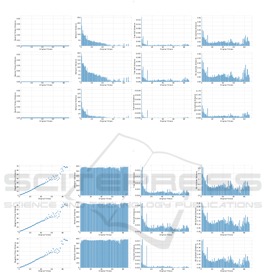
Figure 6: Results after applying subtree (top), structural (middle), and one-point mutation (bottom) for an artificial ant prob-
lem. Original fitness vs neutral fitness (first column), original fitness vs behavior distance (second column), and structural
distance metrics using edit distance (third column) and Weisfeiler-Lehman Subtree Kernel (fourth column).
Figure 7: Results after applying subtree (top), structural (middle), and one-point mutation (bottom) for an artificial ant prob-
lem. Original fitness vs negative fitness (first column), original fitness vs behavior distance (second column), and structural
distance metrics using edit distance (third column) and Weisfeiler-Lehman Subtree Kernel (fourth column).
the genetic operators (Galv
´
an-L
´
opez et al., 2010b). In
our case, there is also an additional peak for a fitness
value of 89. This peak is the result of our static bloat
control, which simply discarded all offspring created
using crossover, which resulted in trees with heights
higher than 20. This resulted in the replication of
highly fit (and possibly bloated) individuals in the lat-
ter stage of the evolutionary process, thus, it is the
result of our sampling method. It is interesting to see
that for subtree and structural mutations, neutral mu-
tations dominate in low fitness range. This changes
above fitness value of 20, where suddenly most of
the mutations have negative effects. In the latter fit-
ness range, neutral and negative mutations occur at a
similar rate. On the other hand, when the one-point
mutation is applied, most of the mutations are neutral
for fitness values lower than 45. Positive mutations
act similarly for all mutation operators. These occur
most frequently in low fitness range and are very rare
for individuals with high fitnesses.
ECTA 2020 - 12th International Conference on Evolutionary Computation Theory and Applications
88

Reversed behavior can be observed for even-6-
parity problems. In this case, most of the mutations
appear for programs with high fitness values (above
half of the maximum fitness, i.e. 32 for even-6-
parity). In this range, neutral and negative mutations
dominate and occur at similar rates. On the other
hand, positive mutations are as frequent as neutral
mutations in the lower half of fitness values. Similar
results were reported in (Galv
´
an-L
´
opez et al., 2010b).
This means that bloat control, which changed the dis-
tribution of fitness values for an artificial ant problem,
did not affect outcomes for even-6-parity problem.
The locality of mutation operators is shown in Fig-
ure 4. Let us start an analysis of the locality of a
mutation operator in a genotype-fitness mapping (top
part of Figure 4). First of all the highest frequency
can be observed for neutral mutations (fitness distance
of 0), regardless of mutation operator. For artificial
ant problem, we can see that it is substantially less
common for mutation operator to introduce big fit-
ness change. This tendency can also be observed for
even parity problem. However, it is far more com-
mon for mutation operation to drastically change the
fitness of the individual in even parity problem. This
is related to the neutral landscape of even parity prob-
lem, for which even small changes of the genotype
can be detrimental for the program.
The locality of mutation operators in genotype-
behavior mapping can be seen in the bottom part of
Figure 4. For even parity problem, the distribution
of behavior distance to the frequency of it occurring,
looks pretty much the same as the distribution of fit-
ness distance. On the other hand, genotype-behavior
mapping presents a completely different view of an
artificial ant problem. Even in this picture, neutral
mutations are most common, however, small behav-
ioral differences are very rare (frequencies at the level
of 10
−5
). Conversely, big behavioral changes (behav-
ior distances close to 600) are very common (around
10
−2
). Frequencies, when fitness distance and behav-
ior distance are 1, are presented in Table 2. Presented
values show that subtree mutation presents the high-
est locality, with the one-point mutation having the
lowest locality. This result is counter-intuitive. The
one-point mutation is the simplest mutation, which
replaces a single node of a tree, thus should have the
highest locality. On the other hand, subtree mutation
is capable of introducing drastic genotypic changes.
This finding is a little bit different from the results
reported in (Galv
´
an-L
´
opez et al., 2010b), in which
structural mutation is shown to have the highest lo-
cality.
Finally, we have to analyze the relation between
fitness and behavior distance to genotypic change in-
troduced through mutations. Cases for positive, neu-
tral, and negative mutations are analysed separately,
and are shown in Figures 5, 6, and 7, respectively.
Due to space restrictions, only results for an artificial
ant problem are presented.
Let us first focus on the results for positive mu-
tations (Figure 5). We can see that on average, the
biggest fitness change is introduced to individuals
with original fitness of around 10. After this point,
the average improvement of an individual’s fitness de-
creases, thus becoming harder to improve programs.
The biggest change can be seen for original fitness
values above 60, where suddenly the distribution be-
comes rugged. These are local optima, which can-
not be easily escaped. It is known that an artificial
ant problem has a highly multimodal landscape, with
many plateaus split by deep valleys (Langdon et al.,
1998). This means that bigger genotypic, as well as
behavioral changes, are required to escape such op-
tima. Similar ruggedness of the landscape can be ob-
served in the following plots for behavioral and struc-
tural distances. In the case of behavior, we can see
that overall behavioral changes (corresponding to fit-
ness improvements) are high, but they also decrease
after the original fitness of 10. This behavior is fairly
natural, that is, to improve individuals with high fit-
nesses we have to optimize their behaviors. However,
when optimal solutions are found (fitnesses > 60),
it is necessary to introduce big changes to the be-
havior (similar to fitness and genotypic changes) to
improve an individual. Similar behavior can be ob-
served for structural changes, which are relatively low
for the whole spectrum of fitness values. However,
this relation becomes rugged in the same region as
for fitness and behavior changes. In the case of tree
edit distance, this relation is harder to see, because
it takes into account only how many edits are nec-
essary to change one tree into another. According
to TED, big behavioral changes are accompanied by
small genotypic changes (only a small subset of nodes
was changed). On the other hand, WL-Subtree kernel
claims that the introduced changes are far greater (on
par with changes introduced for individuals with low
fitnesses).
For neutral mutations, we can observe that big
behavioral changes are recorded for individuals with
low fitness values. These behavioral changes are ac-
companied by relatively high genotypic changes as
shown by both distance measures. On the other hand,
individuals with high original fitnesses, experience
small or no behavioral changes, even for relatively
high genotypic mutations, as given by WL-Subtree
kernel. That is, a highly fit individual cannot drasti-
cally change its behavior if it wants to keep its fitness
Behavioral Locality in Genetic Programming
89

value unchanged. It is worth mentioning, that these
genotypic changes are smaller than the ones observed
for positive mutations (according to WL-Subtree ker-
nel: < 0.2 for neutral and > 0.2 for positive muta-
tions). That is, these changes are small enough not
to escape local optima, as well as, they are not big
enough to enter valleys.
Finally, in the case of negative mutations, we see
that the most detrimental changes can be observed for
individuals with high original fitnesses (> 70). From
the behavioral perspective, all individuals experience
very high changes to their behaviors. This landscape
is stable in comparison to the behavior changes ob-
served for positive mutations. It is interesting to see
that for negative mutations, structural changes are
overall higher than the ones observed for neutral mu-
tations, but are lower than for positive mutations.
5 CONCLUSIONS
Two contributions of this paper are: (i) extending the
definition of GP by considering genotype to behav-
ior mapping; and (ii) proposed to use the family of
similarity measures, Graph Kernels, as a way to cal-
culate genotypic distance. Our proposals were tested
on two benchmark problems, artificial ant and even
parity problem.
First of all, traditionally used Tree Edit Distance
(TED) was compared to the Weisfeiler-Lehman Sub-
tree Kernel. This comparison showed that TED con-
siders trees to be significantly more different than
WL-Subtree kernel. This is due to the way, the
dissimilarity between the trees is calculated, that is
WL-Subtree kernel considers both local (node level)
and global (neighborhoods) properties of trees. This
means that the WL-Subtree kernel uses both syntactic
(structural) and semantic (behavioral) information, to
evaluate dissimilarity.
Investigations on the locality of three basic muta-
tion operators: subtree, structural, and one-point mu-
tations, showed that subtree mutation has the highest
locality. This result is counter-intuitive because sub-
tree mutation changes subtrees (and possibly whole
tree). This result is common for both genotype to fit-
ness and genotype to behavior mappings. However,
for the artificial ant problem, all three mutation oper-
ators have low locality in genotype to behavior map-
ping. That is, the frequency of a highly local change
to occur is much less common than a low locality
change to happen (frequencies at the level of 10
5
vs
10
2
, respectively). In the case of even-6-parity, dis-
tributions of fitness, and behavior distances were ap-
proximately the same.
Finally, our results showed that all mutations are
detrimental to the original behavior of an individual,
regardless of its original fitness and the size of in-
troduced genotypic change. Three considered muta-
tion operators are of low behavioral locality, that is,
they rarely preserve behaviors of programs. There-
fore, even small changes in the genotype, drastically
change an individual’s behavior, thus resulting in
slight improvements or considerable deterioration of
the fitness of an individual. Small behavioral changes
were also recorded, however, these did not change the
fitness of programs.
This work can be extended in several ways. First
of all, it could be applied to a wider variety of prob-
lems, e.g. symbolic regression (both benchmark and
real-world problems), maze navigation, image pro-
cessing, and scheduling. Furthermore, this work ap-
plied the Weisfeiler-Lehman Subtree kernel as a dis-
similarity measure, however, various methods could
also be used, such as, Shortest Path, Random Walk,
Graphlet Sampling, and Laplacian kernels. Finally,
it may be worthwhile to investigate how different
reperesentations of intermediate phenotypes (e.g. bi-
nary decision diagrams) affect the fitness landscape.
REFERENCES
Belea, R., Caraman, S., and Palade, V. (2004). Diagnos-
ing the population state in a genetic algorithm us-
ing hamming distance. In International Conference
on Knowledge-Based and Intelligent Information and
Engineering Systems, pages 246–255. Springer.
Burke, E. K., Gustafson, S., and Kendall, G. (2004). Diver-
sity in genetic programming: An analysis of measures
and correlation with fitness. IEEE Transactions on
Evolutionary Computation, 8(1):47–62.
Burks, A. R. and Punch, W. F. (2015). An efficient structural
diversity technique for genetic programming. In Pro-
ceedings of the 2015 Annual Conference on Genetic
and Evolutionary Computation, pages 991–998.
Galvan-Lopez, E. (2009). An analysis of the effects of
neutrality on problem hardness for evolutionary algo-
rithms. PhD thesis, University of Essex.
Galv
´
an-L
´
opez, E., McDermott, J., O’Neill, M., and
Brabazon, A. (2010a). Defining locality in ge-
netic programming to predict performance. In IEEE
Congress on Evolutionary Computation, pages 1–8.
IEEE.
Galv
´
an-L
´
opez, E., McDermott, J., O’Neill, M., and
Brabazon, A. (2010b). Towards an understanding of
locality in genetic programming. In Proceedings of
the 12th annual conference on Genetic and evolution-
ary computation, pages 901–908.
Gustafson, S. and Vanneschi, L. (2008). Crossover-based
tree distance in genetic programming. IEEE Transac-
tions on Evolutionary Computation, 12(4):506–524.
ECTA 2020 - 12th International Conference on Evolutionary Computation Theory and Applications
90

Jones, T. et al. (1995). Evolutionary algorithms, fitness
landscapes and search. PhD thesis, Citeseer.
Kelly, J., Hemberg, E., and O’Reilly, U.-M. (2019). Im-
proving genetic programming with novel exploration-
exploitation control. In European Conference on Ge-
netic Programming, pages 64–80. Springer.
Koza, J. R. (1992). Genetic programming: on the program-
ming of computers by means of natural selection, vol-
ume 1. MIT press.
Kriege, N. M., Johansson, F. D., and Morris, C. (2020). A
survey on graph kernels. Applied Network Science,
5(1):1–42.
Langdon, W. B. and Poli, R. (2013). Foundations of genetic
programming. Springer Science & Business Media.
Langdon, W. B., Poli, R., et al. (1998). Why ants are hard.
Nikolentzos, G., Siglidis, G., and Vazirgiannis, M.
(2019). Graph kernels: A survey. arXiv preprint
arXiv:1904.12218.
O’Reilly, U.-M. (1997). Using a distance metric on genetic
programs to understand genetic operators. In 1997
IEEE International Conference on Systems, Man, and
Cybernetics. Computational Cybernetics and Simula-
tion, volume 5, pages 4092–4097. IEEE.
Poli, R., Langdon, W. B., McPhee, N. F., and Koza, J. R.
(2008). A field guide to genetic programming. Lulu.
com.
Rothlauf, F. (2006). Representations for genetic and evo-
lutionary algorithms. In Representations for Genetic
and Evolutionary Algorithms, pages 9–32. Springer.
Shervashidze, N., Schweitzer, P., Leeuwen, E. J. v.,
Mehlhorn, K., and Borgwardt, K. M. (2011).
Weisfeiler-lehman graph kernels. Journal of Machine
Learning Research, 12(Sep):2539–2561.
Tai, K.-C. (1979). The tree-to-tree correction problem.
Journal of the ACM (JACM), 26(3):422–433.
Vanneschi, L., Castelli, M., and Silva, S. (2014). A survey
of semantic methods in genetic programming. Genetic
Programming and Evolvable Machines, 15(2):195–
214.
Zhang, K. and Shasha, D. (1989). Simple fast algorithms for
the editing distance between trees and related prob-
lems. SIAM journal on computing, 18(6):1245–1262.
Behavioral Locality in Genetic Programming
91
