
Risk Estimation in Data-driven Fault Prediction for a Biomass-fired
Power Plant
Ivan Ryzhikov
1
, Mika Liukkonen
2
, Ari Kettunen
2
and Yrjö Hiltunen
1
1
Department of Environmental Science, University of Eastern Finland, Yliopistonranta 1, 70210, Kuopio, Finland
2
Sumitomo SHI FW Energia OY, Relanderinkatu 2, 78200, Varkaus, Finland
Keywords: Fault Detection, Feature Creation, Data-driven Modeling, Machine Learning, Risk Estimation, Deep Neural
Network.
Abstract: In this study, we consider a fault prediction problem for the case when there are no variables by which we
could determine that the system is in the fault state. We propose an approach that is based on constructing
auxiliary variable, thus it is possible to reduce the initial problem to the supervised learning problem of risk
estimation. The suggested target variable is an indicator showing how close the system is to the fault that is
why we call it a risk estimation variable. The risk is growing some time before the actual fault has happened
and reaches the highest value in that timestamp, but there is a high level of uncertainty for the times when the
system has been operating normally. We suggest specific criterion that takes uncertainty of risk estimation
into account by tuning three weighting coefficients. Finally, the supervised learning problem with risk variable
and specific criterion can be solved by the means of machine learning. This work confirm that data-driven
risk estimation can be integrated into digital services to successfully manage plant operational changes and
support plant prescriptive maintenance. This was demonstrated with data from a commercial circulating
fluidized bed firing various biomass and residues but is generally applicable to other production plants.
1 INTRODUCTION
The fault prediction problem appears in different
industries. In many cases a fault causes serious
damage to production or business processes, which
comes to a loss of production efficiency and,
consequently, money. Companies need extra
resources to undo the damage of the fault, that is why
preventing the fault is a better practice. By preventing
the fault, we mean having an detection system that
would indicate if the process is of the high fault risk
and we need to do something to prevent the ongoing
fault. This situation is typical for some industries, and
many times a critical process fault can mean a big loss
for the company. In (Paltrinieri and Khan, 2016) the
importance of risk assessment is considered for
chemical industries. Another example is the energy
sector, where any unexpected load limitation or
shutdown of a power unit can cause considerable
economical losses. That is why it is very important to
recognize if the situation is risky that one can prevent
the system from the fault. In fault detection problem
for the power plants there is no single performance
indicator showing how close the system is to the fault.
Rapidly evolving energy market sets challenges to
traditional combustion-based power plants as it
demands efficiency and flexibility in terms of fuel
and load range. For example, the share of biomass as
an energy source has increased significantly during
recent years and it is expected to keep on increasing.
In this paper we consider a real-world problem
concentrating on boiler fault prediction in biomass-
fired circulating fluidized bed (CFB) power plants.
These plants are extremely important and have not
only the financial benefits, but also benefits for the
environment as they can be used to replace fossil-fuel
-based power generation. These plants can utilize
challenging fuels such as biomass or waste residues
efficiently, but the drawback is that these types of fuel
may often cause different problems such as blockages
in the material flow. Especially this concerns biomass
fractions that include large amounts of alkali metals.
Although the consequences of the blockages are
serious, we still cannot measure the quality of the fuel
accurately and need to control the process using the
observational data coming from different other
sensors. In this study we applied the proposed
Ryzhikov, I., Liukkonen, M., Kettunen, A. and Hiltunen, Y.
Risk Estimation in Data-driven Fault Prediction for a Biomass-fired Power Plant.
DOI: 10.5220/0010113104230429
In Proceedings of the 12th International Joint Conference on Computational Intelligence (IJCCI 2020), pages 423-429
ISBN: 978-989-758-475-6
Copyright
c
2020 by SCITEPRESS – Science and Technology Publications, Lda. All rights reserved
423

approach to find patterns in a system state that takes
place priorly to the fault.
Most industrial processes are complex, so they
cannot be designed faultless and cannot be properly
modelled in advance. It is also hard to tell which
observing variables could be used for detection of the
cases when something is wrong with the process.
Moreover, even the process experts cannot always list
the states and conditions by which we could identify
the situations when process could cause the system
fault. If we could have an adequate mathematical
model of the target system, it could be used to predict
the future system state by the inputs and previous
states. In that case, if we know the future system state,
we can predict the fault. But due to complexity of the
production process there is no mathematical model.
But in the case when the most of processes
characteristics are being monitored, we have
observations, that we can use to build data-driven
models.
All the above lead the fault prediction to be based
on analysis of the data that corresponds to stable
functioning and the data that is prior to the fault. The
goal of the prediction system is to identify the patterns
that lead the system to the fault. It is important to
mention that not all the fault prediction problems can
be considered initially as a regression or classification
problems. We consider a case, in which we only know
the time the fault happened and there are only a few
faults occurred during the comparatively large time
interval. Here we need to reduce the initial problem
to regression problem by adjusting the criteria and
auxiliary variable construction. Then we apply
statistical learning methods to the adjusted dataset to
build up a prediction system.
Machine learning algorithms are being widely
utilized to find the relation between the input and the
output of the system (Kuhn and Johnsson, 2016).
There are studies on applying the machine learning
algorithms for solving the fault prediction problem
for supervised learning, but the most of these studies
are focused on specific processes. Since the fault
prediction requires recognition of specific patterns in
data, that cause the system fault, by fault prediction
we would mean the risk estimation problem. By risk
we mean some variable, that indicates the degree of
how dangerous the current situation is, this
interpretation is a simplification of the risk definition
done by (Kaplan and Garrick, 1981), so we are not
estimating the consequences and probabilities. In
(Paltrinieri et. al., 2019) the machine learning based
approach is considered as a promising tool of solving
risk estimation problems. The difference in
approaches is the following: is in that paper there is a
variable that can be used for risk estimation, and in
our case, we need to construct it first. Other
approaches of fault detection can be based on training
model on labelled observations of the system with
and without faults (Bondyra et al., 2018), but these
approaches require observations for both regular and
fault system states. In this study we are interested in
recognition pre-fault state instead of the fault state.
In study (Rakhshani et al., 2009) authors consider
the fault prediction problem for a power plant boiler,
where the risk estimation is based on the dataset with
labeled observations. There is continuous variable
that equals its max value for normal system states and
min value for the faults. The risk estimation is the
prediction of that variable and its values become the
base for the fault detection system. Depending on the
value, the state can be classified as normal, low fault
risk and fault. But it could be too late to prevent the
fault if we detect the fault by the time it has happened
and this case we consider in this paper. It has also
been considered in the study (Hujanen, 2019), where
the problem was reduced to the classification problem
and deep neural networks were applied to find a
model. In this study we propose different approach,
where the risk is assumed to grow constantly starting
from the time prior to the fault. Also, the risk
modeling is adjusted according to uncertainty of the
actual risk level for the observations that is not in this
prior to the fault interval, since there is no prior
information that these observations are of the low or
high risk.
In this paper we describe the reduction of the
initial fault detection problem, the way to construct
the risk variable and adjusted criterion and making
data-driven models. We also discuss the possibility of
using the risk prediction models for identification of
relation between different fault cases.
2 RISK ESTIMATION
APPROACH
Today computational resources allow us to make the
data-driven solutions based on the artificial neural
networks and the other computationally intensive
algorithms (Chollet and Allaire, 2018), (Goodfellow
et al., 2016). These methods and their
implementations are becoming more important in the
era of Industry 4.0 (Brink et al., 2016), when the
collected data could be analyzed and used as
decision-making systems for improving
performance.
The considered process state can be characterized
by different inputs that correspond to the sensor data
NCTA 2020 - 12th International Conference on Neural Computation Theory and Applications
424

from the different parts of the boiler plant. Each of
these inputs can be described as time series with fixed
step size:
,
,…,
,
,
,…,
,
where is a sample size. We also know times at
which the fault happened:
,1,, so we assume
that there had been some time before that, at which
the risk began to grow. This time before the fault is a
parameter ∆ of the proposed approach. We put
forward a hypothesis, that there is no risk in any other
timestamp, than timesteps before the fault limited by
the parameter. We also assume that risk increases
monotonically starting from zero, and it reaches its
maximum value of one by the fault time, so the risk
variable can be evaluated by the following function
,
∆
1,
∆
,
0,,
(1)
where
is the fault time and ∆ is the parameter.
Since there could be different faults, the risk
function for whole observation time can be evaluated
as a sum of single fault functions (1):
,
.
(2)
We assume that there is always a normal system state
between the different faults, so it is possible to find
such ∆that ∄,,
:
∆, so non-zero
intervals of the risk functions are not overlapping.
According to this approach, we need to find a relation
between the system state variables and the risk
feature. In this study we assume that the risk is
increasing identically before any of the faults.
We need to split the data on train and test sets to
estimate the adequacy of model and its
generalization. Since we work with time series,
which consists of several intervals corresponding to
several faults, we consider two splitting schemes.
First option is to leave the data for one of the faults
for the test and to keep other faults data for the train.
This would help us to understand which faults have
similar (or different) patterns corresponding to the
risk increase. Second option is to split the data on two
subsets, one before some date as train and validation
and second after that date as test. In that case we can
see, how good is historical data in predicting the
future faults. To provide validation we used
stratification, so train and validation contain
observations from a common process and
observations from the interval before the fault.
As a modeling criterion we used the root mean
square error
̃
̃
,
(3)
where n is a test or validation subset size,
,
1,
are risks (2) at
timestamps and ̃
,1,
are risk estimations at the same time points by the
model. Since we cannot properly estimate the risk for
the time, when no fault was detected and we cannot
estimate the risk for time intervals right after the
fault, we suggested to use specific weights for these
errors in the sum (3):
̃
∙
̃
,
(4)
where
is a weighting function,
,∈
,
,∈
,
,∈
,
(5)
and
are the time intervals corresponding to
states after the faults,
are the time intervals
before the faults and
are the other intervals.
Here
,
and
are weighing
coefficients. These coefficients are used for
increasing the influence of errors caused at the points,
when the risk was growing and decrease the
influence of errors of risk estimation for the time
intervals for which the risk value is uncertain.
The goal of our risk modelling approach is to
estimate the risk of the current system state and to
observe its dynamics for decision making. It means
that we need to have model with optimal parameters
∗
, which is adequate in risk estimation and thus
minimizing the criterion (4):
̃
|
∗
min
̃
|
,
(6)
where ̃
|
is the model prediction in case of its
parameters . Data-driven model estimates the risk
by process state variables, so
̃
|
̃
|
,
(7)
and
,:
.
The fault prediction problem is reduced to
minimization problem (4), where we use specific
weight coefficients (5). The solution of reduced
problem is optimal model parameters (6), that we use
to estimate a risk by system state variables. Now the
risk estimation can be used for fault prediction and
decision making, but this topic is out of the scope of
the study. In the next chapter we discuss the way we
Risk Estimation in Data-driven Fault Prediction for a Biomass-fired Power Plant
425

transform the state variables into risks (7) by solving
the regression problem (6).
3 DATA-DRIVEN RISK
ESTIMATION
In this study we consider the dataset, a collection of
process variables measurements. We explicitly
selected 54 variables, which, from the experts’ point
of view, could be useful for the fault detection. The
dataset contains 50879 observations and 8 different
process faults. In this study we tried different time
delta parameters and finally used ∆2 hours. In case
of this value and observation step size, there are only
192 observations can be labelled as leading to the
fault. It is typical that the faults occur uniquely, so
there is imbalance between the number of
observations of normal process state and the number
of observations leading to the fault.
We tried different machine learning algorithms,
such as lasso regression, random forests, and
artificial neural networks with different number of
layers and perceptron, still the chosen one is
beneficial. In this study we used deep neural network
with 5 layers, containing 64, 64, 64, 32 and 1
neurons, respectively. We added dropout for the 2
nd
,
3
rd
and 4
th
levels: 0.5, 0.5 and 0.25, respectively. We
used root mean square propagation as a learning
algorithm with a batch size of 5000 and 100
iterations. We used the Keras framework (Allaire and
Chollet, 2018) for modeling, and the application were
implemented in R (R Core Team, 2018). The weighs
(5) for criterion (4) are set as following:
1,
10. The weights were tuned
manually, but these weights tune the model
sensitivity, and the desired sensitivity comes out of
the business needs.
As it was discussed in the previous chapter, we
used two different cross-validation schemes. First,
we use leave-one-out approach for the faults. We
train and validate the model on all the data except the
one of the faults, which is used for the final test.
According to that, we solved 8 different regression
problems, which correspond to 8 different faults. Due
to randomness of the learning algorithms, we solve
each problem 10 times for each case to evaluate the
statistics.
We separated the errors on the ones that model
makes on the common system functioning, and the
error in risk estimation in case of the fault. The
minimum error values for common and risky states
are given in Table 1 and Table 2, respectively.
Table 1: Minimum error in risk estimation of the common
process for cases when one fault is left for test and others
were used to learn the model.
Fault case to test Error minimum (common)
1 1.746891e-05
2 0.0003728659
3 0.0004703251
4 0.0001684821
5 4.076825e-05
6 6.904885e-06
7 0.0001324624
8 5.641435e-05
Table 2: Minimum error in risk estimation of the process 2
hours before the fault for cases when one fault is left for test
and others were used to learn the model.
Fault case to test Error minimum (fault)
1 0.09567184
2 0.1083031
3 0.09283183
4 0.08412199
5 0.1146508
6 0.1078044
7 0.103839
8 0.1143047
As one can see, in Table 1 the average minimum
value is less than 0.0002, but for 2
nd
, 3
rd
and 7
th
faults
the risk estimation for the common state was not
stable. This point will be proved by the risk
estimation visualization below. The results in Table 2
show us, that some faults cannot be predicted by the
model trained on other faults, at least here is no risk
increase at the ∆ interval before the test fault.
Since it is hard to differentiate result only by the
table values, let us visualize the risk estimation for all
the considered problems. Figures 1-8 represent the
risk modeling results in case of different fault cases
used as test.
If we compare Figures and Tables, we can see
that some faults are predicted, since we see the
increase of the risk near the fault time. This increase
happens earlier, than it is being expected: not in ∆
interval prior to the fault. It means that the problems
of this nature require specific metric. Metric which
one can use to estimate if the risk prediction
adequacy is a problem itself. In this study we put
forward a hypothesis that the fault is expected during
the similar time interval prior to the fault. In the
further work we will consider another option of
metric calculation and comparing the modeling
results.
NCTA 2020 - 12th International Conference on Neural Computation Theory and Applications
426
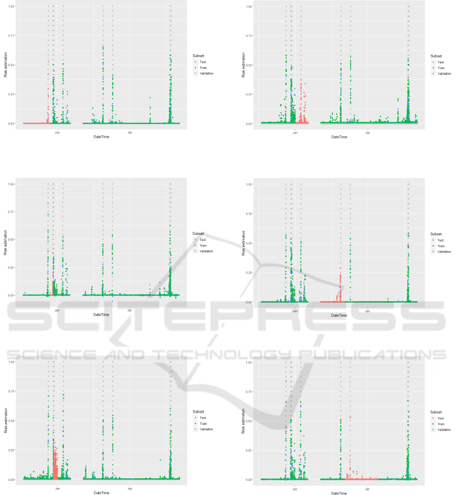
Figure 1: Fault risk estimation in case of the 1
st
fault left for
the test.
Figure 2: Fault risk estimation in case of the 2
st
fault left for
the test.
Figure 3: Fault risk estimation in case of the 3
rd
fault left for
the test.
Figure 4: Fault risk estimation in case of the 4
th
fault left for
the test.
Figure 5: Fault risk estimation in case of the 5
th
fault left for
the test.
Figure 6: Fault risk estimation in case of the 6
th
fault left for
the test.
Risk Estimation in Data-driven Fault Prediction for a Biomass-fired Power Plant
427
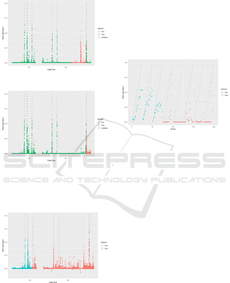
Figure 7: Fault risk estimation in case of the 7
th
fault left for
the test.
Figure 8: Fault risk estimation in case of the 8
th
fault left for
the test.
Now we consider the second validation scheme
in which we use only one third of observations for
train, leaving the rest of the data for the test. For the
same model used we get the results that is presented
in Figure 9.
Figure 9: Risk estimation for the case when we use the
observations before some date as train and leave another
data as test.
This experiment shows us, that the system
predicts some of the faults, but it also shows some
risk increase when there is common process. Of
course, that could happen, because we used only 30%
of data for the train, but even that amount of data is
enough to demonstrate that the proposed approach is
promising. We can see that some of the test faults
caused the risk increase and we also see that this
increase is greater than the one happens by mistake.
To demonstrate the risk estimation right before the
fault, we selected only ∆ intervals and give it in
Figure 10 for train and test.
Figure 10: ∆-interval risk estimations.
In this chapter we examined proposed approach
on solving the real-world biomass and residue fuels
energy station problem. This approach is useful for
analysis of the fault cases and the estimation of the
risk. We considered two different cross-validation
schemes and both schemes demonstrated promising
results.
4 CONCLUSIONS
In this study we proposed the auxiliary risk feature
and used it as a target variable for solving fault
prediction problem. This variable represents the
degree of how close the current situation is to the
fault: the higher the risk is, the closer system is to the
fault. To construct this variable, we used the fault
datetime and the specific time parameter – the time
prior to the fault, when we expect the risk to grow.
Another part of the approach is to provide errors in
risk estimation before the faults being more valuable
for the model learning, than the errors on all the other
intervals, on which the uncertainty is higher. The
weigh parameter values should be tuned so it would
provide the suitable balance between errors of both
types: predicting high risk, when system runs
normally, and predicting no risk, when there is high
risk of the fault. This balance should be determined
by the business needs and out of the scope of this
study.
NCTA 2020 - 12th International Conference on Neural Computation Theory and Applications
428

The proposed approach was applied to solve the
fault detection problem for a CFB process based
power plant burning various type of biomasses.
These systems are expected to benefit from this kind
of risk estimation system, so that one could be able
to detect possible process disturbances in advance to
buy time for remedial actions aimed at preventing a
critical system failure that may eventually lead to a
load limitation or an unexpected shutdown. This
work confirm that data-driven risk estimation can be
integrated into digital services to successfully
manage plant operational changes and support plant
prescriptive maintenance. This was demonstrated
with data from a commercial circulating fluidized
bed firing various biomass and residues but is
generally applicable to other production plants.
Moreover, data-based, digital predictive tools are
expected to play a growing role in the future service
business within the energy production sector as
customers are expecting better availability and
predictability combined with requirement to burn
cheaper and challenging fuels. The considered
approach is useful in revealing the similarities and
differences for the faults and, thus, it is useful for
further monitoring of the system state and for fault
prediction.
As a modeling approach we utilized the deep
neural networks and the results shown in Tables 1
and 2 and on Figures 1-10 demonstrates that the
model gives promising results.
We continue the research by applying another
class of models and using the lagged inputs. Since the
process is continuous and generally its state can be
characterized by the states in the previous
observation points, the promising option would be to
use the convolutional and recurrent neural networks.
The future studies involve developing specific
metric that would help to compare the model
accuracy more precisely. That would allow making
automatic modeling system. Another part of the
future studies is related to the risk time interval
identification since it could be different for all the
cases. Parameter estimation problem can be reduced
to the global optimization problem, that is combined
with modeling, so we will be able to find the risk
parameters and corresponding models
simultaneously.
REFERENCES
Allaire, J.J., Chollet, F., 2018. keras: R Interface to 'Keras'.
R package version 2.2.4. URL https://CRAN.R-
project.org/package=keras
Brink, H., Richards, J., Fetherolf, M., 2016. Real-World
Machine Learning, Manning.
Bondyra A., Gąsior P., Gardecki S. and Kasiński A., 2018.
Development of the Sensory Network for the Vibration-
based Fault Detection and Isolation in the
Multirotor UAV Propulsion System. In Proceedings of
the 15th International Conference on
Informatics in Control, Automation and Robotics -
Volume 2: ICINCO, ISBN 978-989-758-321-6, pp.
112-119. DOI: 10.5220/0006846801120119
Chollet, F., Allaire, J. J., 2018. Deep Learning with R.
Manning. ISBN 978-1-61729-554-6.
Goodfellow, I., Bengio, Y. and Courville, A. 2016. Deep
Learning. MIT Press.
Hujanen, J. Machine Learning Methods for Early Process
Deviation Detection in Circulating Fluidized Bed
Boilers. In: Proc. of Nordic Flame Days 2019.
Kaplan. S., Garrick, B.J., 1981. On the quantitative
definition of risk. Risk Anal., vol. 1, pp. 11-27
Kuhn, M., Johnson, K., 2016. Applied predictive modeling.
Springer
Paltrinieri, N., Comfort, L., Reniers, G., 2019. Learning
about risk: Machine learning for risk assessment. Safety
science, vol. 118, Elseiver, pp 475-486.
Paltrinieri, N., Khan, F., 2016. Dynamic Risk Analysis in
the Chemical and Petroleum Industry, Dynamic Risk
Analysis in the Chemical and Petroleum Industry:
Evolution and Interaction with Parallel Disciplines in
the Perspective of Industrial Application. Butterworth-
Heinemann. 10.1016/B978-0-12-803765-2.01001-5.
R Core Team, 2018. R: A language and environment for
statistical computing. R Foundation for Statistical
Computing, Vienna, Austria. URL https://www.R-
project.org
Rakhshani, E., Sariri, I., Rouzbehi, K, 2009. Application of
data mining on fault detection and prediction in Boiler
of power plant using artificial neural network. 2009
International Conference on Power Engineering,
Energy and Electrical Drives, Lisbon, Portugal
Risk Estimation in Data-driven Fault Prediction for a Biomass-fired Power Plant
429
