Airborne Visual Tracking of UAVs with a Pan-Tilt-Zoom Camera

Athanasios Tsoukalas

, Nikolaos Evangeliou

, Nikolaos Giakoumidis

and Anthony Tzes

Engineering Division, New York University Abu Dhabi, P.O. 129188, Abu Dhabi, U.A.E.

Core Technology Platform, New York University Abu Dhabi, P.O. 129188, Abu Dhabi, U.A.E.

Keywords:

Variable Object Tracking, Visual Homography, Optical Flow.

Abstract:

The visual detection and tracking of UAVs using a Pan-Tilt-Zoom (PTZ) camera attached to another aerial

platform is the scope of this article. The long-term tracker is performing image background subtraction using

visual homography and is used to initialize a short term tracker that works in parallel to enhance the tracking for

various motions. The moving UAV is detected using optical ﬂow concepts and its bounding box encapsulates

its detected features. A Kalman predictor provides a robust smooth tracking of the bounding box in the

temporary absence of a detected UAV. The camera pans and tilts so as the tracked UAV is centered within

its Field-of-View and zooms in order to expand the UAV’s view. Experimental results are offered using an

evader-tracker UAV-group to validate the presented tracking algorithm.

1 INTRODUCTION

In this work the subject of the Long Term Tracking

(LTT) of a target UAV from another one equipped

with a Pan - Tilt - Zoom (PTZ) camera is consid-

ered. The estimation of the strong background im-

age feature points in comparison to those of a mov-

ing object is performed through a comparison of the

image optical ﬂows and the predicted position of the

feature points according to the Homography transfor-

mation derived between feature points found in pre-

vious frame and the estimate in the current frame.

A Kalman prediction ﬁlter (Paul and Musoff, 2015)

can smooth the trajectory in the presence of noisy

measurements, while a correlation based tracking al-

gorithm is also used in combination with our LTT

scheme to account for the cases where the UAV

blends with the background.

Previous research on Variable Object Tracking

(VOT) has focused on strong image features matching

and Homography. In (Eshel and Moses, 2008) mul-

tiple static cameras are used to infer multiple mov-

ing targets, using the homography of three planes

parallel to the ﬂoor between each pair of cameras.

In (Arr

ospide et al., 2010) the ground plane is de-

tected using a single moving camera, by ﬁnding the

homography between the ground planes in successive

images, using a feature matching approach. These

methods assume that the ﬂoor or a top down view

is always present in the camera view. In (Cui et al.,

2019) a moving object segmentation is performed

from stationary or moving cameras based on homog-

raphy constraints across multiple frames, that de-

scribes the background motion, without assuming a

planar scene using a pixel precision. In (Dey et al.,

2012) the detection of independently moving fore-

ground objects in non-planar scenes captured by a

moving camera is performed, using a multi frame

monocular epipolar constraint of camera motion. The

method applies optical ﬂow across the whole image

between consecutive frames, that scales exponentially

in performance loss as the image resolution is higher.

In (Viswanath et al., 2015) foreground object seg-

mentation is performed with a background modelling

technique that models each pixel with a single Spatio-

Temporal Gaussian. In (Sheikh et al., 2009) objects

are tracked using a freely moving camera with no

assumptions that the background approximated by a

plane, by building a sparse background model by es-

timating a compact trajectory basis from trajectories

of salient features across the video. Following the

background subtraction by removing trajectories that

lie within the space spanned by the basis, builds the

foreground and background appearance models. Then

an optimal pixel-wise foreground/background label-

ing is obtained by efﬁciently maximizing a posterior

function. In (Fu et al., 2016) the algorithm tracks

by ﬁnding feature correspondences in a way that an

improved binary descriptor is developed for global

feature matching, while an iterative Lucas–Kanade

Tsoukalas, A., Evangeliou, N., Giakoumidis, N. and Tzes, A.

Airborne Visual Tracking of UAVs with a Pan-Tilt-Zoom Camera.

DOI: 10.5220/0010112900900097

In Proceedings of the International Conference on Robotics, Computer Vision and Intelligent Systems (ROBOVIS 2020), pages 90-97

ISBN: 978-989-758-479-4

optical ﬂow algorithm is employed for local feature

tracking and a local geometric ﬁlter (LGF) module

maintaining pairwise geometric consistency is used to

identify outliers.

In all of the above methods (excluding (Viswanath

et al., 2015)), the feature points are identiﬁed and

matched between frames, resulting in one extra step

dependent on both the feature matching between

frames algorithm and the feature selection algorithm.

In our method we do not perform any feature match-

ing, using directly the positions estimated by the op-

tical ﬂow as next-frame features and calculate the

homography matrix based on the features found in

the previous frame and the estimated by the optical

ﬂow in the current frame. This allows for a one-

to-one correspondence of features positions between

frames, removing any ambiguity as to which fea-

tures are matched and dramatically enhances perfor-

mance as there is no need for a feature matching step.

In (Viswanath et al., 2015), similar to our method the

feature points in the previous frame are tracked using

an optical ﬂow method and a Homography is calcu-

lated for the background pixels, under the assump-

tion of an initial background state image and subse-

quently updating a distribution of background proba-

bility of each pixels in the new frame. This is used to

model the new background and perform background

subtraction using the entire new background image

as mask, requiring a signiﬁcant computational bur-

den.This method does not behave well in the absence

of many background points to estimate the Homogra-

phy, and the foreground object estimation needs more

computations, since it operates on the whole image

for both the background transformation/subtraction.

In Section 2 the visual tracking problem of the

UAV from another airborne UAV statement is pro-

vided, followed by the case of identifying a ﬂying

object using the Homography based method in Sec-

tion 2.1. In Section 3 the method of estimating the im-

age based optical ﬂow is discussed using the current

and previous image frames. In Section 4 the method

of estimating the image ﬂow for background image

features based on the Homography transformation de-

rived between image feature points found in previous

and current frames is discussed as well as the method

of comparing the two ﬂows in order to evaluate which

parts of the image are background, that is when the

optical ﬂow velocity vectors match closely those of

the expected by the Homography based ﬂow estima-

tion of the image features corresponding to the back-

ground. The method of calculation of the bounding

box around the tracked target UAV points that have

been identiﬁed as foreground is also discussed. In

Section 5 the implementation of the Kalman predic-

tor for the smooth follow of the tracked UAV dur-

ing tracking window estimation noise is discussed. In

Section 6 a correlation based tracker is considered and

described, for further enhancing the ability to track

the object when the ﬂow based method is not pro-

viding a result due to object blending with the back-

ground. In Section 7 the control of the PTZ camera

motion to track the target UAV is discussed along with

the overall algorithm. In Section 8 the results of an

experiment of tracking a UAV from a ﬂying UAV pur-

suer is presented and analyzed.

2 AIRBORNE

VISUAL-TRACKING OF UAV

The algorithms are running locally on a mini i7-based

Intel NUC PC on board of an enhanced Vulkan UAV

shown in Figure 1.

Figure 1: Tracker UAV with mounted PTZ-camera.

Real time LTT of an object using a video-stream is

a complex task due to the limited information we have

about the object. The various correlation methods

give a good tracking performance, given the motion

is not very fast and can keep the correlation strong

between frames, but fail when the motion is fast and

loose the tracking window. These must be initial-

ized with a starting window that engulfs the object

to track. Thus a LTT-scheme based on object motion

is required in order to track a general object across

all motions regions, occlusion and change of appear-

ance. Such a scheme is proposed in this article, en-

hanced with a correlation based tracker for the cases

where the object blends with the background since its

motion which can be slow or not moving relative to it.

2.1 Object Tracking Method using

Homography

The background subtraction method used in order

to identify the moving object motion is relying

only on visual feedback and homography calcula-

Airborne Visual Tracking of UAVs with a Pan-Tilt-Zoom Camera

tions (Szeliski, 2010) between two frames. This

method is robust against general disturbances and per-

forms well when IMU measurements are not avail-

able. Initially a strong image features set is identi-

ﬁed on the previous camera frame and an optical ﬂow

technique is used to estimate the position of the fea-

tures in the current frame, as shown in Figure 2. The

method involves the discovery of special image areas

with speciﬁc characteristics. The feature set is a col-

lection of pixel points in the camera image, while var-

ious algorithms are available for the discovery of im-

age features (Tareen and Saleem, 2018).

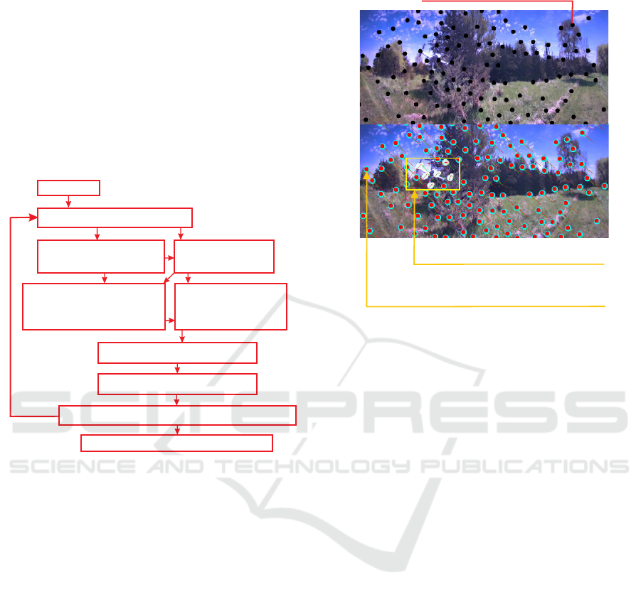
0: Initialize

1: Get current image I

2: Detect corner features

in I

3: Calculate optical

ﬂow from toI I

4: Calculate Homography

using features computed in

steps 2 and 3

5: Identify foreground

features

i-1

6: Dilation of moving points

7: Bounding box calculation

8: Bounding box prediction using Kalman ﬁlter

9: PTZ-camera PID control for VOT

Figure 2: Visual Homography based tracking.

OpenCV’s “goodFeaturestoTrack” (Shi and

Tomasi, 1994) algorithm was used for ﬁnding the

strong corners image features in our experiments

Under the assumption that the background holds the

majority of the pixels with a consistency in displace-

ment, a homography is calculated that transforms the

features positions from the previous to the current

frame, which correspond to the background pixels.

The previous frame features are then transformed

using the homography to get their position in the

current frame. We assume that the background points

transformed with the homography that corresponds

mainly to the background pixels group will coincide

with the estimated ones by the optical ﬂow, while

the moving objects features estimated by the optical

ﬂow will diverge from the homography transformed

pixels, as shown in Figure 3.

The pixels that correspond to static background

objects will follow the predicted motion by the Ho-

mography transformation and coincide to the po-

sitions predicted by an optical ﬂow based estima-

tion, while the rest will be classiﬁed as belonging to

Estimated UAV bounding box

after background points removal

Optical ﬂow and Homography based estimated

positions of features in the current frame

in red and cyan respectively.

Feature points positions

in previous image frame

Brightness of circles is proportional to divergence

of the two estimates of features position.

(When 0 assume features are on background)

≈

Figure 3: Homography/Optical ﬂow tracking method.

moving objects of interest (Figure 4). The calcula-

tions of the optical ﬂow follow the Lucas - Kanade

method (Lucas and Kanade, 1981) with an extension

using a pyramidal scheme with variable image resolu-

tions (Bouguet, 2000). The basic optical ﬂow premise

is to discover the position of an image feature from

previous frame, in the current frame.

One downside of the technique is that when the

tracked object remains static and blends with the

background, it cannot be identiﬁed, thus a correlation

short term tracker relying on the MOSSE tracking al-

gorithm (Bolme et al., 2010) is used. This identiﬁes

the UAV’s position until new estimated positions from

the ﬂow based method are available. The beneﬁt of

the LTT-schemer is that requires zero a priori infor-

mation, unlike the methods that require prior knowl-

edge of the target bounding window for initialization.

2.2 Homography Calculation

The homography or perspective transform can be for-

mulated as a 3 × 3 operator H on homogeneous coor-

dinates









= H ˜x =

















. (1)

The resulting homogeneous coordinates x

, y

are nor-

malized as

ROBOVIS 2020 - International Conference on Robotics, Computer Vision and Intelligent Systems

t-1

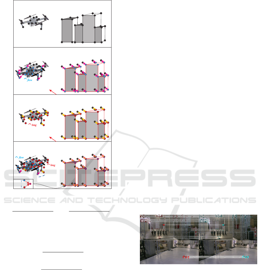
Target drone

Static Background

Image features in frame t-1

Camera motion

Estimated features in frame using optical ﬂow based

on the drone position

Estimated features in frame using Homography

transformation

Estimated background - foreground features in frame t

d > threshold

d ≈ 0

Background

Foreground

ﬂow

hmg

Figure 4: Foreground identiﬁcation method.

+ h

, y

+ h

, (2)

while the operator H is calculated such that minimizes

the back projection error

∑



−

+ h





−

+ h



. (3)

In order to get a good estimation of the transfor-

mation matrix in the presence of outliers, which may

include foreground points that move not inline with

the background point majority, the RANSAC method

is used to estimate the homography matrix using this

subset followed by a simple least-squares algorithm to

compute the quality of the computed homography (de-

ﬁned by the number of inliers). The best subset is then

used to produce the initial estimate of the homography

matrix. The computed homography matrix is reﬁned

further with the non linear Levenberg-Marquardt opti-

mization (Levenberg, 1944; Marquardt, 1963) method

to further reduce the re-projection error.

3 OPTICAL FLOW ON SPARSE

IMAGE FEATURES

When the tracker UAV is moving, static camera based

background subtraction algorithms cannot provide an

accurate UAV-tracking, and another background sub-

traction method needs to be implemented for this case.

The method involves the discovery of special image ar-

eas with speciﬁc characteristics in the camera image,

which we note as the image feature set F

at time t. The

feature set is a collection of pixel points in the camera

image p

= [px

, py

]. Various algorithms are available

for the discovery of image features (Tareen and Saleem,

2018).

OpenCV’s “goodFeaturestoTrack” (Shi and Tomasi,

1994) adapted to run on the GPU using the “se-

tUseOpenCL” of the OpenCL module and UMat image

holder is employed to ﬁnd the strong corners image fea-

tures. This algorithm calculates the corner quality mea-

sure at every source image pixel using the Minimum

Eigenvalue or the Harris method. For each of the dis-

covered image features of the previous image frame, the

optical ﬂow F

is derived as a collection of velocity vec-

tors that correspond to each of the image features. For

the optical ﬂow estimation of the discovered image fea-

tures, the OpenCV function “calcOpticalFlowPyrLK” is

used. The method operates on a sparse feature set using

the iterative Lucas-Kanade method with pyramids and

the inputs are the current and previous frames as well as

the image features identiﬁed from the previous frame.

The output is the estimated feature position in the cur-

rent frame. An example of the feature matching between

the current and previous frames is presented in Figure 5.

Figure 5: Image feature matching between successive

frames.

The algorithm also provides a status ﬂag for each

point that describes whether a ﬂow was found for the

speciﬁc point. The calculations of the optical ﬂow fol-

low the Lucas - Kanade method (Lucas and Kanade,

1981) with the an extension using a pyramidal scheme

with variable image resolutions (Bouguet, 2000). The

basic optical ﬂow premise is to discover the positioning

of an image feature in the previous frame, in the current

captured frame.

OpenCV’s calcOpticalFlowPyrLK function is used

accepting as inputs the previous camera image, and the

feature points selected in the previous image to estimate

Airborne Visual Tracking of UAVs with a Pan-Tilt-Zoom Camera

the optical ﬂow on the current camera image. The output

is the estimated points along with status number for each

estimation, which has a value of one if an estimation of

the point in the new image is found, otherwise is zero.

4 HOMOGRAPHY-BASED

TRACKING

The tracking method differentiates the foreground to the

background image features discovered in the previous

image frame. The estimated background points given by

the transformation of those points using a Homography

matrix are compared to the foreground ones and their

estimated positions by an optical ﬂow method, in the

current frame.

Given an image g

t−1

in time t − 1, we derive the es-

timation of the positions of the selected image feature

points set F

in the image g

in time t, based on the Ho-

mography calculated between the strong feature points

of the previous and current camera frames, as described

in the previous sections. Then an optical ﬂow method

as described in Section 3 is used for the same estimation

of the feature point positions. The two resulting posi-

tions are compared to distinguish the background points

from the moving ones, considering the estimation points

with distance less than a threshold would belong to the

background. The optical ﬂow provides the estimation

ˆp

f low

of the position of a feature point in the previous

frame g

t−1

, in the current frame g

for the p

point in

the previous frame and an estimation of the point ˆp

Hmg

is also provided from the Homography based transfor-

mation on the feature points set of the previous frame

t−1

. The distance b

= || ˆp

f low

− ˆp

Hmg

|| is evaluated

and if b

) ≥ b

bkgd

, ∀p

∈ F

(image feature point set),

then the point p

is considered as moving, otherwise as

a background one.

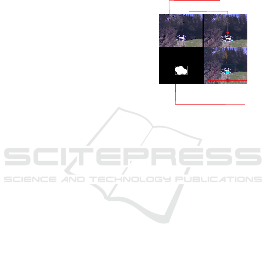
The foreground points correspond to those describ-

ing the UAV; a dilation operator followed by the compu-

tation of a predicted bounding around the blob of points

that surrounds the UAV, as shown in Figure 6 bottom

left window, using OpenCV’s function “Find Contours”

in combination with the “approxPolyDP” function that

approximates found contours with polylines that are in-

serted into the “boundingRect” function to create the

bounding box around the polyline. The aforementioned

search is performed at each frame and the performance

of the system using a 960 × 540 pixels is at 65fps on

the airborne i7 CPU Intel NUC PC. The NUC’s GPU

is used with OpenCL library for OpenCV to enhance

the performance of the optical ﬂow and image manip-

ulation calculations. When the background has static

objects across a wide range of distances to the tracker

UAV, some points may be identiﬁed as foreground, thus

a second background layer is assumed and the Homog-

raphy is recalculated using this new subset, in order to

identify the remaining background points. It should be

noted that this layer can be computed extremely fast due

to the lack of need to compute the optical ﬂow.

Estimated UAV bounding box

after background points removal

and dilation of the foreground

points

Estimated image feature points

corresponding to the UAV

Strong image feature points

Figure 6: Estimated image features on tracked UAV.

5 KALMAN FILTER TRACKING

OF BOUNDING BOX

A Kalman ﬁlter prediction scheme tracks the motion

smoothly in the absence of a tracking window (or short

time sensor malfunction) in some frames and provides

the an estimate of the UAV’s trajectory. The Kalman

predictor uses a state vector X = [x, y, ˙x, ˙y, ¨x, ¨y, w, h]

comprising of the position (Velocity) of the center of

the tracking window [x, y] ([ ˙x, ˙y), and the width and

height of the window w, h. The estimated vector m

, y

, ˙x

, ˙y

, w

, h

] contains the currently identiﬁed

window center x

, y

, its velocity ˙x

, ˙y

and box’s

width and height w

, h

. The ˆx

-estimate of X is found

in a recursive manner as

ˆx

= F

ˆx

k−1

= F

k−1

+ Q

Under the assumption of a constant acceleration, the

state transition matrix is







dtI







where dt is the time delta between two consec-

utive frames, and I

) is the 2 × 2 identity

(zero) matrix . The expected process noise covari-

ance matrix of the model is assumed to be Q =

diag(σ

, σ

˙x

, σ

˙y

, 0, 0, σ

, σ

). The conversion of the

state space to measurement units is performed through

the measurement adaptation matrices m

= H

ˆx

, and

ROBOVIS 2020 - International Conference on Robotics, Computer Vision and Intelligent Systems

= H

, where









For our tracking window measurements, we deﬁne

= diag(σ

, σ

˙x

, σ

˙y

, σ

) as the covari-

ance of the estimated window parameters measurement

noise induced uncertainty and z

the mean of the mea-

surements. The ﬁnal measurement update ˆx

and the

covariance

are deﬁned as

ˆx

= ˆx

t−1

+ K(z

− H

ˆx

) (4)

= P

t−1

− KH

t−1

(5)

where the Kalman gain K is given by

K = P

+ R

)

−1

(6)

The measurement matrix is updated with the esti-

mated bounding box position-width-height and velocity

calculated using the position estimations in previous and

current frames and the time between them.

6 CORRELATION BASED MOSSE

TRACKING ALGORITHM

In the case where a UAV is hovering, the optical ﬂow

method may not provide results as essentially the UAV

can be considered as background. To avoid this behav-

ior we use the MOSSE tracking algorithm (Bolme et al.,

2010) around the tracking window to check if the cor-

relation to the previous frame stays strong, and decide

whether to keep the window to the same position or

move it to some other position, according to the latest

measurements. The MOSSE algorithm requires an ini-

tial bounding box around the target, which we provide

through our LTT when the conﬁdence is high enough

across multiple frames and the MOSSE tracking win-

dow to our estimated tracking window have distance be-

yond a threshold. A weight is given based on how strong

the correlation and how far the new measurement from

the previous to make the ﬁnal decision. When MOSSE

algorithm alone is used to track the target UAV, the re-

sults are generally adequate, but the algorithm needs an

initial tracked object bounding box and also can fail to

provide information for the loss of tracking, getting lo-

cally trapped in an image position different than the re-

quired one. Thus an LTT-scheme is needed for MOSSE

re-initialization in loss of tracking. The MOSSE algo-

rithm uses the correlation of a ﬁlter calculated by the

previous bounding box engulfed image and the current

image, to track closeness of the current frame to the ini-

tial target provided by the LTT. The calculations are per-

formed using FFT, due to the fact that correlation can be

expressed as the element wise multiplication of the in-

dividual FFT on the correlation ﬁlter and current image.

Thus the correlation between the input image F = F(f )

and the ﬁlter H = F(h) is expressed as

G = F  H

∗

. (7)

The ﬁlter is initially trained by the UAV image,

provided by the optical ﬂow based method that deter-

mines the initial tracked object bounding box. The tar-

get is then tracked by correlating the current ﬁlter over a

search window in the next frame and the maximum cor-

relation output position indicates the new position of the

target. The ﬁlter is then retrained based on the newly

identiﬁed position. The ﬁlter is deﬁned such that it min-

imizes the square error sum between the actual and de-

sired output of the convolution.

min

∗

∑

 H

∗

− G

. (8)

resulting in

∗

∑

 F

∗

 F

∗

. (9)

The numerator can be interpreted as the correlation

between the input and the desired output and the de-

nominator is the input energy spectrum. The training

set is constructed using random afﬁne transformations

to generate eight small perturbations ( f

) of the track-

ing window in the initial frame. Training outputs (g

)

are also generated with their peaks corresponding to the

target center. During tracking, a UAV-target can often

change appearance by changing its rotation, scale, pose,

by moving through different lighting conditions. There-

fore, ﬁlters need to quickly adapt in order to follow ob-

jects. Running average is used for this purpose. The it-

erative MOSSE ﬁlter after the initialization is computed

∗

 F

∗

+ (1 − n)A

i−1

 F

∗

+ (1 − n)B

i−1

(10)

where n is the learning rate. MOSSE’s performance

ws found to be suitable for real time tracking. In Fig-

ure 6, the MOSSE tracking window is shown in blue box

around the tracked UAV. The Kalman tracking window

is represented by the red box and the magenta one cor-

responds to the predicted tracking object bounding box

by the optical ﬂow and Homography method.

7 PTZ CAMERA CONTROL

The PTZ camera moves according to commands issued

by its programming API. A PID controller has been de-

vised to track the discovered target UAV by turning the

camera towards the UAV with the goal to center it on the

screen at every frame. When the target has been near

centered, a zoom action is performed in order to extend

the target’s bounding box thus eliminating a portion of

the background that may affect the tracking result. The

overall algorithm for tracking a target UAV is presented

in the sequel.

Airborne Visual Tracking of UAVs with a Pan-Tilt-Zoom Camera

1: Initialize algorithm and retrieve ﬁrst frame I

2: Retrieve current image I

and buffer I

i−1

3: Detect the coordinates (x, y) of image feature set

i−1

, in previous frame I

i−1

4: Calculate the optical ﬂow from I

i−1

to I

such that

i−1

corresponds to the g

features.

5: Estimate background pixels position ˆg

for every

i−1

feature using Homography transformation.

6: Subtract ˆg

from the optical ﬂow g

to get estima-

tion distance b

= || ˆp

f low

t+1

− ˆp

Hmg

t+1

||.

7: The feature points p

in g

where b

) ≥

bkgd

∀p

∈ g

are considered moving, otherwise these

are marked as background.

8: Dilate the foreground points and extract the

polygonal boundaries around point concentrations.

9: Generate bounding boxes around identiﬁed fea-

tures clusters and select the largest one that corresponds

to the tracked object.

10: Initialize and run in parallel the MOSSE corre-

lation based tracker when the measurements conﬁdence

is high across multiple frames.

11: Use a Kalman ﬁlter to smoothly track the

MOSSE estimated tracking window in each frame.

12: Use the PID controller to direct the PTZ to the

tracked object.

13: Repeat step 2.

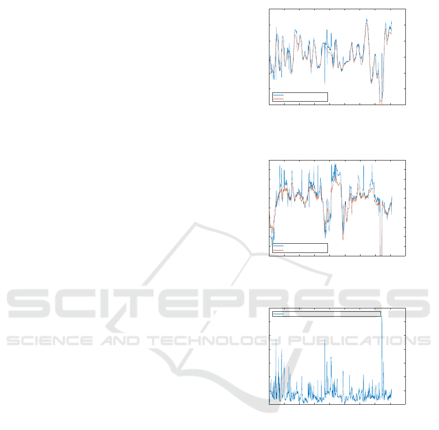
8 EXPERIMENTAL STUDIES

The results of an airborne tracking of a UAV is presented

in this section. Both UAVs are monitored by a Motion

Capture System (MoCaS) using a set of 24 Vicon cam-

eras. Figures 7 to 9 show the tracking results in pix-

els. It is shown that the tracking using the Homogra-

phy based method closely follows the tracked UAV and

is further enhanced when the MOSSE correlation based

tracking is also used to account for the cases where there

is no position estimate. The MOSSE algorithm is re-

initialized based on the measurements by our method,

given a conﬁdence of three consecutive frames with an

estimated object position that does not diverge beyond

a threshold. In the case where no measurement track-

ing window or MOSSE tracking window is estimated,

the previous known estimation is used respectively. A

presentation of the algorithm working on smooth mo-

tion videos and multiple targets can be previewed in the

videos in (Tsoukalas, 2020).

9 CONCLUSIONS

A method to determine the trajectory of a moving UAV

has been presented in this work, using a PTZ camera.

The foreground is discriminated from the background

based on the comparison of the predicted background

0 200 400 600 800 1000 1200 1400 1600 1800

Video Frame

200

400

600

800

1000

1200

Tracked object average position - X axis

Tracked object X axis average position from Measurement and MOSSE tracked estimations

MOSSE-Measurement Average

Vicon

Figure 7: Estimation of X axis of the tracked UAV using

MOSSE and Measurements estimations.

0 200 400 600 800 1000 1200 1400 1600 1800

Video Frame

100

150

200

250

300

350

400

450

500

550

Tracked object average position - Y axis

Tracked object Y axis average position from Measurement and MOSSE tracked estimations

MOSSE-Measurement Average

Vicon

Figure 8: Estimation of Y axis of the tracked UAV using

MOSSE and Measurements estimations.

0 200 400 600 800 1000 1200 1400 1600 1800

Video Frame

100

200

300

400

500

600

700

Tracked object distance to Vicon measured real position

Distance of averaged estimated tracked object position to Vicon measurement

MOSSE and Measurement average position to Vicon positions distance

Figure 9: Distance betwen Tracked UAV estimated position

and MoCaS real position.

image features motion using the Homography derived

by image feature sets between two successive frames

and the motion estimated by the optical ﬂow between

these frames. The optical ﬂow long term tracking and a

correlation short term tracking are combined to provide

a robust tracking scheme. A Kalman predictor is also

used in order to smoothly follow the trajectory and in-

crease the tolerance of the system to the tracked UAV’s

bounding box prediction temporal errors.

ROBOVIS 2020 - International Conference on Robotics, Computer Vision and Intelligent Systems

REFERENCES

Arr

ospide, J., Salgado, L., Nieto, M., and Mohedano, R.

(2010). Homography-based ground plane detection

using a single on-board camera. Intelligent Transport

Systems, IET, 4:149 – 160.

Bolme, D., Beveridge, J., Draper, B., and Lui, Y. (2010). Vi-

sual object tracking using adaptive correlation ﬁlters.

In Proceedings of the IEEE Computer Society Con-

ference on Computer Vision and Pattern Recognition,

pages 2544–2550.

Bouguet, J. Y. (2000). Pyramidal implementation of the

lucas kanade feature tracker. Intel Corporation, Mi-

croprocessor Research Labs.

Cui, Z., Jiang, K., and Wang, T. (2019). Unsupervised

moving object segmentation from stationary or mov-

ing camera based on multi-frame homography con-

straints. Sensors, 19:4344.

Dey, S., Reilly, V., Saleemi, I., and Shah, M. (2012). De-

tection of independently moving objects in nonplanar

scenes via multi-frame monocular epipolar constraint.

In Computer Vision – ECCV 2012, pages 860 – 873.

Eshel, R. and Moses, Y. (2008). Homography based multi-

ple camera detection and tracking of people in a dense

crowd. In 2008 IEEE Conference on Computer Vision

and Pattern Recognition.

Fu, C., Duan, R., Kircali, D., and Kayacan, E. (2016). On-

board robust visual tracking for UAVs using a reliable

global-local object model. Sensors, 16:1406.

Levenberg, K. (1944). A method for the solution of cer-

tain non-linear problems in least squares. Quarterly

of Applied Math., 2(2):164–168.

Lucas, B. and Kanade, T. (1981). An iterative image regis-

tration technique with an application to stereo vision.

In Proceedings of the 7th International Joint Confer-

ence on Artiﬁcial Intelligence, volume 2, pages 674–

679.

Marquardt, D. (1963). An algorithm for least-squares es-

timation of nonlinear parameters. SIAM Journal on

Applied Mathematics, 11(2):431–441.

Paul, Z. and Musoff, H. (2015). Fundamentals of Kalman

Filtering: A Practical Approach. American Institute

of Aeronautics and Astronautics.

Sheikh, Y., Javed, O., and Kanade, T. (2009). Background

subtraction for freely moving cameras. Proceedings of

the IEEE International Conference on Computer Vi-

sion, pages 1219–1225.

Shi, J. and Tomasi, C. (1994). Good features to track. In

Proceedings of IEEE Conference on Computer Vision

and Pattern Recognition, pages 593–600.

Szeliski, R. (2010). Computer Vision: Algorithms and Ap-

plications. Springer-Verlag, Berlin, Heidelberg, 1st

edition.

Tareen, S. A. K. and Saleem, Z. (2018). A comparative anal-

ysis of sift, surf, kaze, akaze, orb, and brisk. In 2018

International Conference on Computing, Mathemat-

ics and Engineering Technologies (iCoMET), pages

1–10.

Tsoukalas, A. (2020). Tracking videos using Homography

based algorithm. https://drive.google.com/open?id=

1MgL1RoW7r36ftm aloNzV GJstS4L7Wr.

Viswanath, A., Behera, R., Senthamilarasu, V., and Kutty,

K. (2015). Background modelling from a moving

camera. Procedia Computer Science, 58:289–296.

Airborne Visual Tracking of UAVs with a Pan-Tilt-Zoom Camera