Traffic Flow Modelling for Pollution Awareness: The TRAFAIR
Experience in the City of Zaragoza
Sergio Ilarri
1 a
, David S
´
aez
2
and Raquel Trillo-Lado
1 b
1
I3A, University of Zaragoza, Zaragoza, Spain
2
University of Zaragoza, Zaragoza, Spain
Keywords:
Traffic Flow Modelling, SUMO, Data Management, Sensor Data.
Abstract:
Performing a suitable traffic monitoring is a key issue for a smart city, as it can enable better decision making
by both citizens and public administrations. For example, a city council can exploit the collected traffic data
for traffic management (e.g., to define suitable traffic policies along the city, such as restricting the circulation
of traffic in certain areas). Similarly, citizens could use those data to take appropriate mobility decisions.
To measure traffic, a variety of detection methods can be used, but their widespread deployment through the
whole city is expensive and difficult to maintain. Therefore, alternative approaches are required, that should
allow estimating traffic in any area of the city based only on a few real traffic measurements.
In this paper, we describe our approach for traffic flow modelling in the city of Zaragoza, which we are
currently applying in the European project “TRAFAIR – Understanding Traffic Flows to Improve Air quality”.
The TRAFAIR project aims at the development of a platform to estimate the air quality in different areas
of a city, and for this purpose traffic data plays a major role. Specifically, we have adopted an approach
that combines historical real traffic measurements with the use of the traffic simulator SUMO on top of real
roadmaps of the city and applies a trajectory generation strategy that complements the functionalities of SUMO
(e.g., SUMO’s calibrators). An experimental evaluation compares several simulation alternatives and shows
the benefits of the chosen approach.
1 INTRODUCTION
Pollution is a major source of health problems (e.g.,
see (Curtis et al., 2006; Anenberg et al., 2018)) and
traffic is a major cause of urban pollutants released
into the atmosphere (e.g., see (Mayer, 1999; Samet,
2007; La
˜
na et al., 2016)). Motivated by this, we are
currently working, within the context of the European
project TRAFAIR - Understanding Traffic Flows to
Improve Air quality (2017-EU-IA-0167) (TRAFAIR
Team, 2018; Po et al., 2019), and in close cooper-
ation with a national project that tackles data man-
agement challenges (TIN2016-78011-C4-3-R, “Data
4.0: Challenges and Solutions – UZ”), in the devel-
opment of a platform to provide information and pre-
dictions related to air quality in several cities in Eu-
rope, which implies, among others, the deployment
of low-cost air quality sensors, data collection and in-
tegration, modeling and prediction, the publication of
a
https://orcid.org/0000-0002-7073-219X
b
https://orcid.org/0000-0001-6008-1138
open data, and the development of applications to ex-
ploit the data collected. Among the different types of
data that must be collected and integrated, traffic data
can be highlighted due to the clear impact of traffic on
pollution.
Traffic flow modeling and management is indeed a
critical issue for smart cities (Sharif et al., 2017; Dja-
hel et al., 2015; Anastasi et al., 2013). However, usu-
ally it is not possible to accurately monitor the flow of
cars in every road segment of a city, as this would re-
quire an expensive sensor infrastructure that should be
deployed and maintained. Instead, the traffic is mea-
sured only at some key points of the city, by deploy-
ing suitable sensors there, and other techniques can
be applied to extrapolate the traffic measurements to
other areas of the city. For this, a traffic flow model
can be defined to try to estimate traffic flows in the
whole city that are compatible with the few available
real observations. Simulation tools, fed with the traf-
fic measurements collected by real traffic sensors, can
be used to obtain the potential traffic flows.
One possibility to estimate traffic flows could be
Ilarri, S., Sáez, D. and Trillo-Lado, R.
Traffic Flow Modelling for Pollution Awareness: The TRAFAIR Experience in the City of Zaragoza.
DOI: 10.5220/0010110501170128
In Proceedings of the 16th International Conference on Web Information Systems and Technologies (WEBIST 2020), pages 117-128
ISBN: 978-989-758-478-7
Copyright
c
 2020 by SCITEPRESS – Science and Technology Publications, Lda. All rights reserved
117

to use a traffic simulator. For example, VanetMo-
biSim (H
¨
arri et al., 2006; H
¨
arri et al., 2011) is a Java-
based simulator focused on vehicular ad-hoc net-
works (VANETS) (Ilarri et al., 2015), which supports
both macroscopic and microscopic simulations. As
another alternative, MAVSIM (Urra and Ilarri, 2016)
is a simulator specifically designed to test applica-
tions for VANETS that are based on the use of mobile
agent technology (Trillo et al., 2007) for distributed
data management. These types of simulators allow
the application of different types of vehicle mobility
models (H
¨
arri et al., 2009; Camp et al., 2002), such
as the Random Waypoint Model (RWM), the Graph-
Based Mobility Model (GBMM), the Constant Speed
Motion (CSM) model, and the Smooth Motion Model
(SMM), which allow a simulation of traffic at the in-
dividual vehicle level (microscopic simulations), but
they do not support combining those mobility models
with real input traffic data.
In order to have realistic simulations that are con-
sistent with real traffic observations obtained by the
available traffic sensors, it is essential to be able to
feed real traffic data as an input to a traffic simula-
tion. SUMO (Simulation of Urban MObility) (Kra-
jzewicz et al., 2002; Behrisch et al., 2011) is a popular
simulator, which supports the definition of calibra-
tors (German Aerospace Center (DLR), Institute of
Transportation Systems, 2020c) to regulate the traffic
in specific segments according to the expected traf-
fic values. In this paper, we use and evaluate SUMO,
considering both microscopic and mesoscopic simu-
lations and complementing SUMO’s built-in capabil-
ities (such as the use of calibrators) with other simu-
lation strategies for traffic regulation. There are also
simulators that consider communication network as-
pects in the simulations, such as VEINS (Vehicles in
Network Simulator) (Sommer, 2006; Sommer et al.,
2011), which is an open source software that supports
the re-routing of vehicles based on network messages
received, and is based on SUMO for the simulation of
traffic and OMNeT++ (OpenSim Ltd., 2000) for the
simulation of network communications; however, in
our case, we do not need to simulate network com-
munication aspects, as we are only interested in the
mobility of vehicles.
In this paper, we describe our experience with the
development of a traffic flow modelling approach for
the city of Zaragoza in Spain. The structure of the rest
of this paper is as follows. In Section 2, we describe
the types of available traffic data that are collected in
the city of Zaragoza. In Section 3, we present our
approach for traffic modelling in TRAFAIR. In Sec-
tion 4, we present the experimental evaluation that
we have performed to assess the validity and bene-
fits of our modelling approach. Finally, in Section 5,
we present our conclusions and some future research
directions.
2 TRAFFIC INPUT DATA
In this section, we describe the traffic data sources
available. First, in Section 2.1, we focus on travel
time and average speed data about some routes of the
city, that can be obtained thanks to a system based on
capturing data from Bluetooth devices. Then, in Sec-
tion 2.2, we consider historical traffic data provided
by other types of detectors (inductive coils and pneu-
matic tubes connected to traffic counters).
2.1 Travel Time and Average Speed
Data
The City Council of Zaragoza has Bluetooth antennas
distributed around the city for traffic measurement,
using Worldsensing’s Bitcarrier Traffic Flow Manage-
ment technology (Worldsensing, 2018; Worldsensing,
2020). Besides, several “links” have been defined as
specific routes from one antenna to another antenna
(see Figure 1 for an example): the average speed of
the vehicles that went through a link within a specific
time interval (5 minutes) is computed by consider-
ing the distance between the antennas and the time
needed by the vehicles to traverse that link. Based
on these data, the municipality of Zaragoza provides
a traffic map (see Figure 2) that offers information
about three different levels of traffic in some road
segments of the city (https://www.zaragoza.es/ci
udad/viapublica/movilidad/trafico/trafico.htm),
distinguishing among fluid traffic, dense traffic, and
congested traffic, by using different colors. Besides,
some icons are used to indicate roadworks and other
possible incidents. It also publishes as open data (at
https://www.zaragoza.es/sede/portal/datos- abie
rtos/servicio/catalogo/291), in JSON format (http:
//www.zaragoza.es/trafico/estado/tiempos.json), real-
time traffic information containing the travel time of
certain routes (the origin and destination are described
in natural language, each usually represented as an in-
tersection of two roads and/or popular points of inter-
est in the city).
These data may allow defining a partially-filled O-
D (origin-destination) matrix with some travel times.
However, they are insufficient for our purposes, as
only some routes of the city are covered and the data
available concerns only the travel time; instead, we
need data about the numbers of vehicles in as many
road segments as possible. More specifically, the data
WEBIST 2020 - 16th International Conference on Web Information Systems and Technologies
118

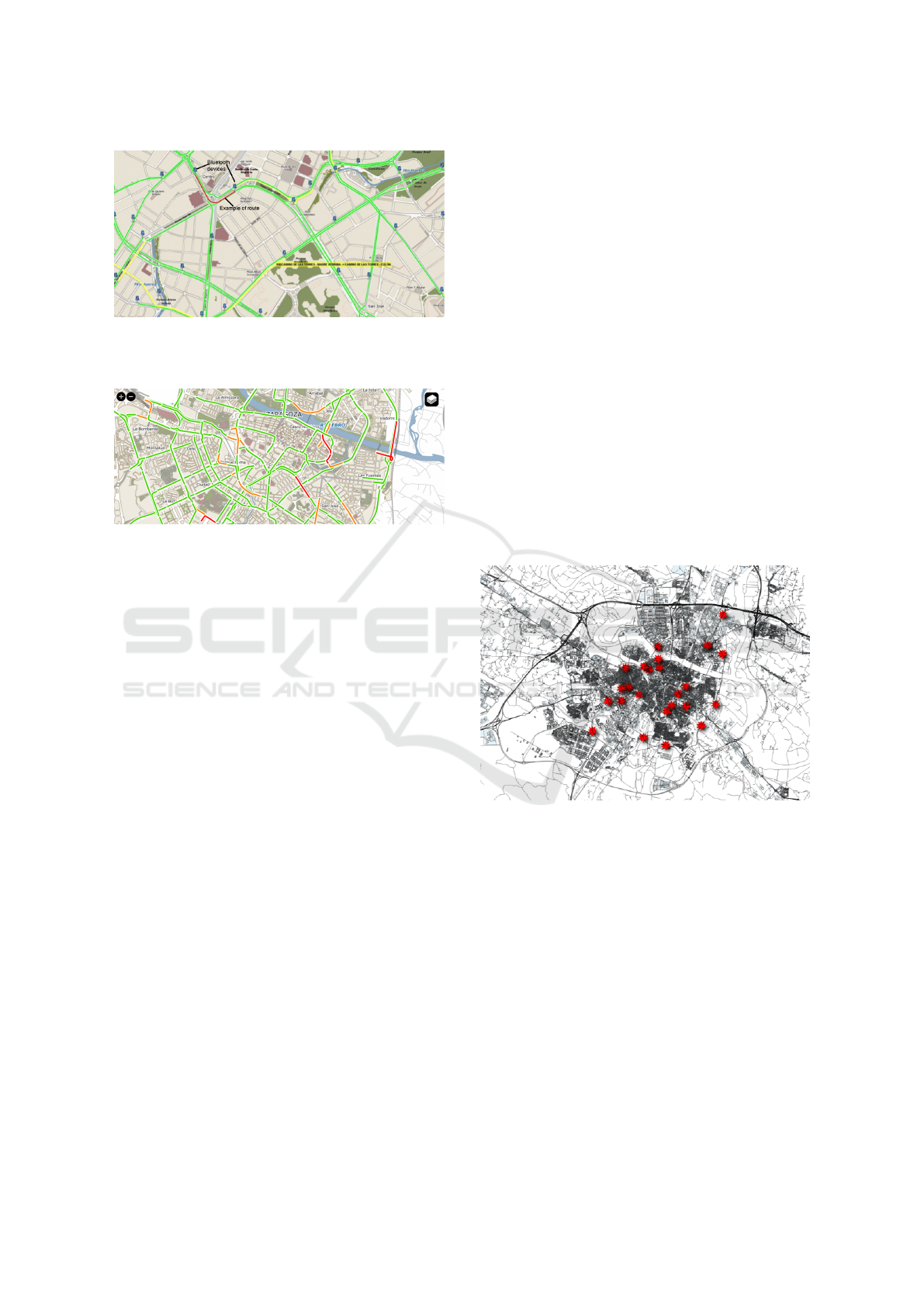
Figure 1: Example of a route whose average travel speed
is measured using Bluetooth devices (City Council of
Zaragoza).
Figure 2: Snapshot of a portion of the real-time traffic map
provided by the website of the City Council of Zaragoza
(data as of March 27, 2020, at 12:40).
in the website are updated every 30 seconds, but they
cover only some routes in the city of Zaragoza; for
example, a query submitted on March 25, 2020, re-
turned only 24 routes (while if we use the data about
the static traffic sensors described in Section 2.2 we
have precise traffic counts of 46 road segments). Nev-
ertheless, this information could be used to feed the
SUMO traffic model with real-time travel time data
in order to refine a traffic model. However, including
these data is not direct and an in-depth analysis of the
current strategy would be required, since as an input
to SUMO we need data about the number of vehicles
on the road segments.
Similarly, the traffic information provided by
Google Maps (Google, 2020) offers an overall view of
the traffic density in different areas of a city (a green
color is used to represent no traffic delays, orange is
used for a medium amount of traffic, and red indi-
cates traffic delays –the darker the red, the slower the
traffic–) as well as information related to several types
of traffic incidents (accidents, constructions, road clo-
sures, and other incidents). Besides, there is an op-
tion to visualize either the live traffic or the typical
(expected) traffic. It covers many streets in the city
of Zaragoza (although some secondary streets are not
currently considered, according to what we have ob-
served on March 11, 2020). Besides, it does not
provide fine-grained traffic information such as the
counts of vehicles on different road segments.
2.2 Traffic Counts Data
Nevertheless, the Zaragoza Traffic Control Center
also provides us with some historical data obtained by
both traffic static devices and traffic mobile devices
measuring the traffic flow of different road segments
in the city:
• Static traffic devices (called “permanent stations”
or “estaciones permanentes” in Spanish) are 46
devices installed in different positions of the
city of Zaragoza (see Figure 3, generated using
QGIS (QGIS Development Team, 2004), where
the static traffic devices are marked in red). These
devices are inductive coils located under the as-
phalt and they provide data about the traffic dur-
ing 24 hours a day for all the days in a year, which
is the reason why they are said to be “permanent”.
Usually, there are two devices in the same traffic
road, one for each direction of circulation. How-
ever, in a few exceptions (specifically, for two
cases) there is only one device measuring the traf-
fic in just one direction (see Figure 4).
Figure 3: Static traffic devices in the city of Zaragoza (snap-
shot of QGIS).
• Mobile traffic devices (termed “annual stations”
or “estaciones anuales” in Spanish) are mobile de-
vices installed in different points of the city along
the year (in an overall of 546 different locations
in 2019). More specifically, they are pneumatic
tubes on the roads connected to traffic counter de-
vices. Usually, there are two devices on the same
road (one for each direction of circulation), as it
is the case for static devices, but there are also
exceptions. These is a set of predefined loca-
tions where these mobile devices can be located
but in each location there is a device measuring
traffic only for a few days (an average of 3 days
with a standard deviation of 0.63), as the static
devices are moved around these defined locations
Traffic Flow Modelling for Pollution Awareness: The TRAFAIR Experience in the City of Zaragoza
119

Figure 4: Example of two static devices measuring traffic on two road segments in just one direction (maps provided by
OpenStreetMap; screenshots of the spatial data viewer of the DBeaver tool, available at https://dbeaver.io).
from time to time. The predefined locations are
called “annual stations” because the devices in-
stalled there try to predict the average annual traf-
fic density in work days (“Intensidad Media Lab-
orable” –IML–).
Using these historical traffic data (for the moment, we
have official historical traffic data for the whole 2018
and 2019), we can feed SUMO with the information
needed to build our traffic model, which is able to es-
timate the traffic for each road segment of the city at
any time instant.
3 TRAFFIC MODELLING
APPROACH
In Figure 5, we show an overview of our traffic
modelling approach, based on the use of the open-
source simulation software SUMO (Simulation of Ur-
ban MObility) (Krajzewicz et al., 2002; Behrisch
et al., 2011). The goal of the traffic model is to es-
timate traffic data on each road segment of the city
(specifically, the number of vehicles passing through
that road segment during each hour of the day and
their average speed) based on a limited set of ob-
served data (real traffic observations on only a few
road segments –in our current prototype, the segments
where there is a static traffic device–). In this way, we
can obtain an overall picture of the traffic in any part
of the city without the need to install sensors along
all the road segments, which would be very expen-
sive; instead, we only exploit the data captured by the
already-existing sensors installed in the city. Our traf-
fic model takes several inputs in order to obtain a traf-
fic flow for the whole city:
• A roadmap representing the city. We have down-
loaded the roadmap of the city of Zaragoza
from OpenStreetMap (OpenStreetMap Founda-
tion (OSMF), 2004) in OSM (OpenStreetMap)
format. Then, we have stored this roadmap in
the TRAFAIR database (including, besides the
road graph, elements such as the number of lanes
and speed limit of each road section, turn restric-
tions, the presence of traffic lights, etc.), to en-
able its easy use by the different components of
TRAFAIR. As a Database Management System
(DBMS) we are using PostgreSQL (The Post-
greSQL Global Development Group, 1996) with
the PostGIS (PostGIS Team, 2001) extension to
handle spatial data.
• Historical data provided by static traffic sensors.
As described in detail in Section 2, and partic-
ularly in Section 2.2, we exploit historical traf-
fic data provided to us by the Municipality of
Zaragoza, captured by the so-called “permanent
stations” (static traffic devices).
• A date, for which we want to estimate the traf-
fic flows throughout the city. This data could be
a past day or a future date. When the input is
a past day for which real traffic observations are
available, the traffic model will estimate the traf-
fic in all the road segments of the city based on
the available real observations. If the input is a
future date, then the traffic model will try to pre-
WEBIST 2020 - 16th International Conference on Web Information Systems and Technologies
120

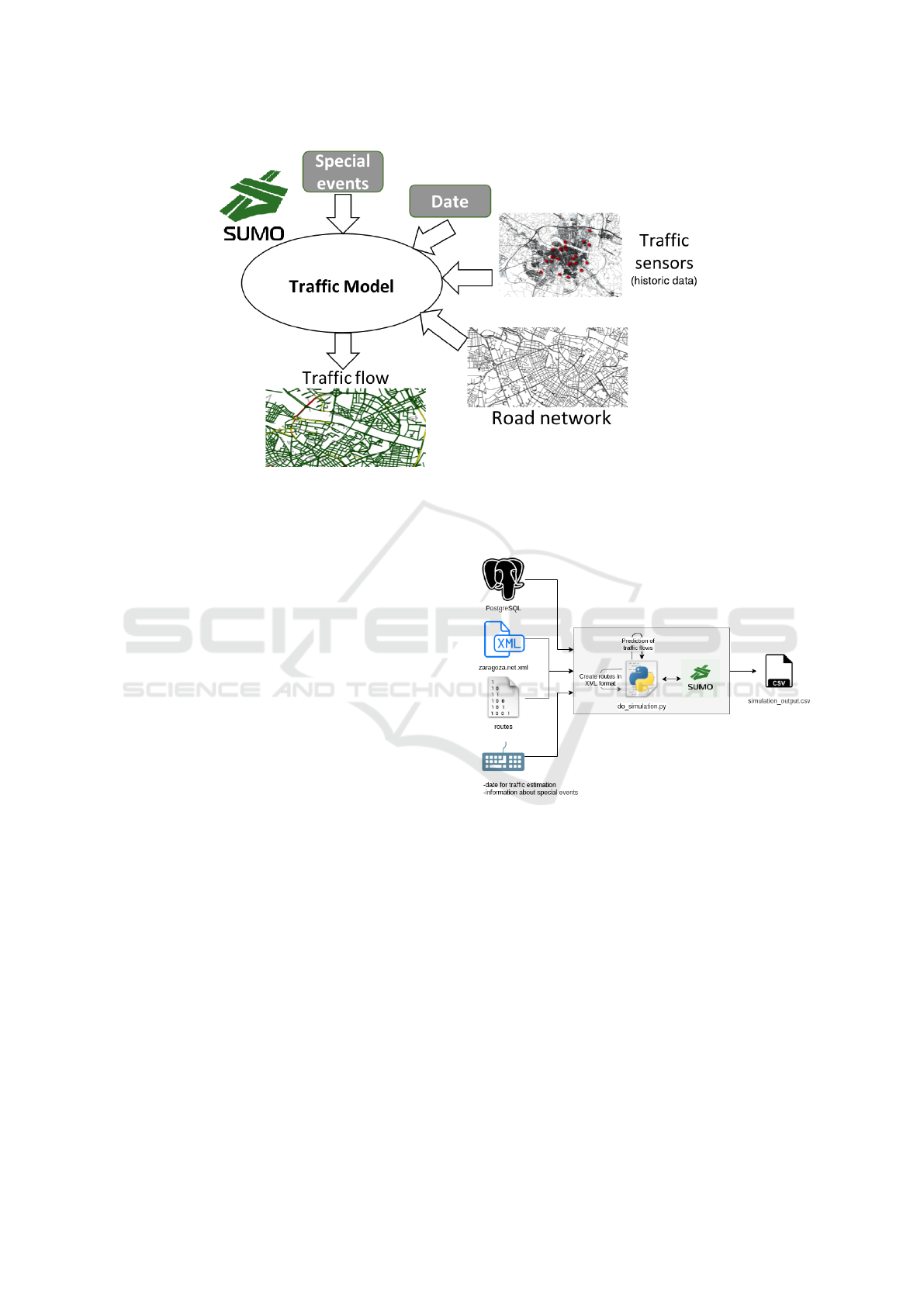
Figure 5: Overview of the traffic modelling approach.
dict the traffic in the city during that day based on
the historical data available.
• Information about special events, which could re-
quire fine-tuning some parameters of the models
generated. For example, during the onset of the
COVID-19 crisis, strict transportation constraints
severely limited the existing traffic in many cities.
This situation changed as the constraints started
to be relaxed as the resolution of the crisis pro-
gressed; indeed, with the pandemics, existing traf-
fic may aggravate due to the potential preference
for single-occupancy vehicles as opposed to pub-
lic transportation (Hu et al., 2020). Overall, as
these are unexpected situations, the impact of
these events may lead to traffic following trends
quite different from the ones observed in the past.
Therefore, this input to the traffic model is used to
adjust the models based on this information, for
example, by automatically reducing the expected
traffic in Zaragoza by a certain percentage during
the first weeks of the state of alarm/emergency de-
creed in Spain due to the COVID-19; as an exam-
ple, according to TomTom’s data, Madrid’s traffic
decreased then by 96% (Dickson, 2020).
The workflow defined for the generation of traffic data
for a given date is shown in Figure 6. A Python
script is in charge of handling the input parameters
described above, interacting with SUMO, and retriev-
ing the results from SUMO in CSV format. The out-
put CSV contains a row for each road segment and
hour during the day; each row includes fields such as
the edge identifier (a road segment or edge is a street
or a part of a street, as defined by the edges in Open-
StreetMap), the hour of the day, the number of ve-
hicles passing through that segment at that hour, and
their average speed.
Figure 6: Workflow used to estimate traffic for a given date.
In Figure 7, we show the workflow defined for
the creation of a roadmap in the format required by
SUMO. First, a Python script queries the TRAFAIR
database, to obtain information about the roadmap of
Zaragoza, and generates a file with the roadmap in
OSM format. Then, another Python script takes the
OSM file and transforms it into a roadmap file com-
patible with SUMO, by using the SUMO tool netcon-
vert (German Aerospace Center (DLR), Institute of
Transportation Systems, 2020a).
For the simulation of traffic with SUMO, three
components have been defined and implemented:
• A traffic predictor, whose goal is to predict the
expected traffic flow that will be measured by the
traffic stations on a (future) date for which real
data are not (yet) available. For this purpose, a
Traffic Flow Modelling for Pollution Awareness: The TRAFAIR Experience in the City of Zaragoza
121

Figure 7: Workflow used to create a roadmap in the format
required by SUMO.
multiple linear regression (Aiken et al., 2012) is
applied on the real historical observations pro-
vided by the traffic stations for all the dates in
our historical dataset (for the work performed in
this paper, we use historical data corresponding
to the dates between January 1, 2018 until March
24, 2019). Based on these historical data and a
number of variables/predictors that we have pre-
viously defined, we have obtained an adjusted R
2
of 0.7736 (more than 75% of the variance is ex-
plained by the model). As predictors, we use the
id of the traffic station, the real traffic data ob-
served by that traffic station, and the month, hour,
and type of day (weekday, Saturday, or holiday)
for that observation.
• A route generator, which computes routes that
can be used by the vehicles within the SUMO
simulation (see Figure 8). Notice that the actual
routes followed by the vehicles are not available
input data, as we only have information about the
traffic flows at specific locations in the city. The
strategy used for the generation of routes is as fol-
lows. First, for each traffic monitoring device,
all the possible routes passing through the road
segment attached to that device (which we call
the target road segment) are computed; to avoid
lengthy computations, a maximum route length
is considered (in our prototype, 30 edges), such
that only the routes passing through the consid-
ered road segment and smaller than the maximum
route length are actually computed. Besides, the
minimum amount of time needed to reach the tar-
get road segment following that route (which we
call the route latency) is computed: this mini-
mum time can be estimated considering that the
car moves through each road segment at its max-
imum allowed speed and that all the traffic lights
along the route are green. The output of this pro-
cess is, for each traffic monitoring station, a list of
possible eligible routes passing by that station.
• A route allocator, which randomly assigns routes
pre-calculated by the route generator to vehicles
during a simulation with SUMO. The assignment
of routes should be compatible with the traffic ob-
servations at each traffic monitoring station. For
example, if during the hour of the day that is be-
ing simulated at the moment there are 200 vehi-
Figure 8: Workflow used to generate possible routes to be
used by vehicles in SUMO.
cles that should pass by station EP2.1, then we
have to generate 200 vehicles and assign to each
of them a route that passes by that station (ran-
domly selected among the pre-computed routes
for that station). In our current prototype, all
the pre-computed routes whose route latency is
smaller than one hour are eligible, but the prob-
ability that a specific route is selected increases
with the number of road segments it contains (in
order to minimize the number of short routes gen-
erated) and with the presence of major city roads
such as avenues or main roads along the city (as
routes traversing those popular roads are more
likely). Furthermore, the route allocator tries to
distribute the passage of vehicles by each station
as uniformly as possible during the hour that is
being simulated, as this is usually more realis-
tic than having large peaks of traffic at specific
moments within the hour; for this purpose, for
each traffic monitoring station, each hour is di-
vided into 3600/numVehicles intervals (seconds
per vehicle), where numVehicles is the total flow
of vehicles expected to be detected by that station
during that hour; then, during each of those inter-
vals one vehicle is scheduled to pass by that sta-
tion (the moment when each vehicle should start
its trajectory is estimated based on the origin of its
route and the time when it is scheduled to pass by
the traffic monitoring station).
Besides, the use of the previous components are com-
bined with the use of SUMO calibrators (German
Aerospace Center (DLR), Institute of Transportation
Systems, 2020c), which are devices that try to reg-
ulate the amount of traffic passing through the edge
where they are located according to the expected traf-
fic flow specified for that calibrator (through an in-
put XML file). In our case, we attach one calibrator
to each edge where a static traffic monitoring station
is located and assign to the calibrator a target traffic
WEBIST 2020 - 16th International Conference on Web Information Systems and Technologies
122

flow equals to the expected traffic flow on that road
segment (i.e., the real traffic observation, if available,
or the predicted traffic flow otherwise). SUMO cal-
ibrators apply an algorithm, described in (Erdmann,
2012), to insert or remove vehicles, as needed, when
it is expected that the target traffic flow will not be
reached. It is possible to assign random or fixed
routes to the additional vehicles that may be inserted
by SUMO: we have decided to use random routes for
those vehicles.
The use of calibrators represents a complemen-
tary strategy to the use of our defined route allocator.
Thus, notice that the route allocator operates under
uncertainty, which may lead to sub-optimal results.
On the one hand, as route allocators act independently
for each traffic station, the impact of the allocations
performed by one route allocator are not considered
by the other route allocators when performing their
allocations: as a route passing by one station may also
pass by other stations, this may lead to an increased
number of vehicles for some stations. On the other
hand, the real route latency can actually be larger than
the one estimated (e.g., due to traffic jams), which
could decrease the final number of vehicles passing
by a given station. These effects can be minimized
thanks to the use of calibrators. Although it is possible
to use only calibrators and the randomTrips.py script
of SUMO to generate routes randomly, the use of our
own route trajectory generator and allocator gives us
more control over the final trajectories followed by
the individual vehicles.
4 EXPERIMENTAL EVALUATION
In this section, we present an experimental evalua-
tion that we have performed to assess our approach
using SUMO to generate a traffic model for the city
of Zaragoza.
In the literature, three types of traffic flow mod-
els have been identified (Krauß, 1998): microscopic
models, mesoscopic models, and macroscopic mod-
els. SUMO provides two of these types of models,
which we have compared in our experiments:
• Microscopic Simulations (Chowdhury et al.,
2000; Lopez et al., 2018). The default simula-
tion model of SUMO implies performing a mi-
croscopic simulation, where the dynamics of each
vehicle are modelled individually.
• Mesoscopic Simulations (Eissfeldt, 2004). A
mesoscopic model combines features of micro-
scopic simulations and macroscopic simulations
(that focus on average vehicle dynamics like the
traffic density). Specifically, the mesoscopic
model of SUMO, which is based on the work
presented in (Eissfeldt, 2004), “computes ve-
hicle movements with queues and runs up to
100 times faster than the microscopic model of
SUMO” (German Aerospace Center (DLR), In-
stitute of Transportation Systems, 2019a).
In the rest of this section, we present the details of the
experimental evaluation. In Section 4.1, we explain
the main metrics that have been considered for eval-
uation, and in Section 4.2 we show some results ob-
tained. Besides the experimental tests and the scripts
implementing the traffic modelling approach defined,
we have also developed a GUI for end users (a ver-
sion of this GUI is currently accessible at http://atil
a.unizar.es:8082/), which supports basic interaction
and visualization of the traffic flows in a user-friendly
way. The user selects the input data and can also in-
dicate optional information in case there is some spe-
cial event in the city that can affect the expected traffic
flows. As an example, in Figure 9, we show a snap-
shot of the traffic flow map computed for a day with
a special event that implies traffic higher than usual.
The map is interactive, and so for example the user
can move around the map, zoom in or out, or click
on a specific location to obtain details (as an example,
see Figure 10).
4.1 Evaluation Metrics
We consider two main evaluation metrics:
• The simulation error. As commented before, we
have some real traffic data measured/expected in
some specific streets of the city and our traffic
model must estimate the traffic in all the streets of
the city by simulating the flow of vehicles along
the roads. Therefore, a key evaluation metric to
consider is the absolute hourly simulation error,
which is the difference between the real traffic
measured in the streets that are being monitored
(i.e., covered by one of the 46 static traffic de-
vices) and the traffic generated in the simulation
with SUMO, for each hour. For example, if the
static traffic device EP2.1 has measured 500 cars
in an hour but in the simulation only 420 cars pass
by that station, then the simulation error for that
hour is 80 cars.
Ideally, the simulation error should be 0. How-
ever, as the amount of real observations is small,
we have to artificially generate realistic trajecto-
ries throughout the whole city based on the real
observations, which will lead to some errors in the
streets where the traffic is being monitored.
Traffic Flow Modelling for Pollution Awareness: The TRAFAIR Experience in the City of Zaragoza
123

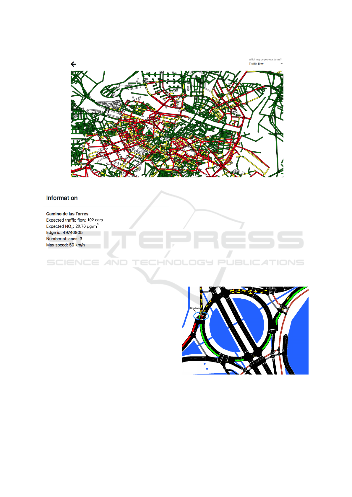
Figure 9: Traffic flow simulation for an expected special event.
Figure 10: Data shown for a position clicked on the map.
A simulation error of n vehicles could be consid-
ered large, medium, or small depending on how
big this number is in comparison with the real
number of vehicles that have been observed. It
is therefore convenient to be able to interpret the
absolute simulation error in relative terms. Specif-
ically, the simulation error rate for a given hour in
the day and static traffic device can be computed
by dividing the absolute simulation error for that
device and hour by the real observation (i.e., the
real traffic demand at that station and time).
• The number of teleports. SUMO avoids poten-
tial simulation deadlocks and undesirable situa-
tions by automatically teleporting vehicles that
have been waiting (without moving) for a while
in front of an intersection (by default, 5 minutes)
or that suffer a collision (German Aerospace Cen-
ter (DLR), Institute of Transportation Systems,
2019b). As an example, a deadlock between two
vehicles is shown on the left part of Figure 11 (the
vehicles are represented as triangles in the GUI
of SUMO): the green vehicle wants to enter the
roundabout and the red vehicle wants to exit it, but
each vehicle waits for the other to move in order to
avoid a potential collision, which leads to a dead-
lock that will only be solved by teleporting one of
the vehicles. We can consider teleports as a sim-
ulation hack used to guarantee that the simulation
will keep progressing in a suitable way, but obvi-
ously automatic displacements of vehicles along
the roads are not desirable, even though SUMO
considers the average speed of the edges when
performing the teleporting and the vehicle is rein-
serted into the network as soon as this becomes
possible (i.e., when there is enough space on the
target lane). Therefore, the number of teleports
should be as small as possible.
Figure 11: Deadlock between two vehicles at the entrance
of a roundabout in Zaragoza during a SUMO simulation.
It should be noted that many of those dead-
locks can be solved by manually editing the road
network (file .net.xml) by using the graphical
network editing tool netedit (German Aerospace
WEBIST 2020 - 16th International Conference on Web Information Systems and Technologies
124

Center (DLR), Institute of Transportation Sys-
tems, 2020b) provided by SUMO (e.g., to change
the priority of the lanes, add lanes, etc.). However,
this leads to a solution which is prone to errors
(the real layout must not be changed, even if that
change avoids the deadlocks), time-consuming
(each problematic point must be carefully edited
by a human), and difficult to maintain (as the pro-
cess cannot be automated, if we download an up-
dated roadmap then all the changes have to be re-
applied manually over the new up-to-date map).
Through experimentation, we have observed that
the number of teleports is particularly high in the
case of microscopic simulations. We have also
observed that the trends regarding the number of
teleports vary along the day: as expected, peak
hours (when the number of vehicles circulating
is high) lead to higher numbers of deadlocks and
therefore to more teleports. The likelihood of
teleports can be reduced by manually editing the
maps through a trial-and-error procedure: when
a simulation bottleneck is observed, causing tele-
ports, we can try to fix it by editing the map. For
example, by manually editing 71 intersections in
the city of Zaragoza, we could reduce the number
of teleports in a typical day from a total of 1860
to 81. However, as commented before, a manual
editing of the map has several disadvantages.
4.2 Experimental Results
First, we compared mesoscopic simulations with mi-
croscopic simulations and noticed that mesoscopic
simulations lead to a smaller number of errors in
terms of the final traffic flows obtained when com-
pared with the expected traffic flows at the locations
with traffic monitoring stations. As an example, the
maximum hourly error (maximum value of the dif-
ferences between the expected traffic flows and the
simulated traffic flows during each hour of the day
at the edges with monitoring stations) for the 21st
of June, 2020, was 300 with the mesoscopic simu-
lation and 2638.4 with the microscopic simulation;
the corresponding average relative error rate (average
values of those differences computed as percentages
over the expected traffic flow at each edge) was 1.34%
with the mesoscopic simulation and 10.55% with the
microscopic simulation. The simulation errors along
that day can be seen in Figure 12, which shows how
the simulation error rates increase with the number
of vehicles (i.e., during the peak hours) when a mi-
croscopic model is used; however, with the meso-
scopic model there are variations but the error rate
keeps quite stable along the day. Only in the cases
of a very low flow of vehicles the microscopic sim-
ulation has low errors comparable to those obtained
with the mesoscopic simulation (even slightly lower
in some cases, like at 6:00 and at 22:00).
Regarding the number of teleports, we have also
noticed that the percentage of teleported vehicles with
a microscopic simulation is considerably higher than
with a mesoscopic simulation. Besides, we have ob-
served that the microscopic model is quite more sensi-
tive to small changes in the road layout (e.g., the pres-
ence or absence of traffic lights in a roundabout can
lead to deadlocks that are solved by SUMO through
teleporting). Figure 13 shows the percentage of ve-
hicles teleported along the day when a microscopic
simulation is used. Again, we can observe that the
number of errors increases with the number of vehi-
cles (i.e., the error is higher during the peak hours).
The previous experimental results advise the use
of mesoscopic simulations rather than microscopic
simulations, and therefore we use the former in our
current prototype. Thus, we have also performed sev-
eral experiments focusing only on mesoscopic simu-
lations. As an example, Figure 14 shows the relative
error rate and the rate of teleports for the simulation
of one week of traffic, since Monday (June 15, 2020)
until Sunday (June 21, 2020); we can see that the er-
ror rates are quite small. Besides, they both decrease
significantly during the weekends, which are the peri-
ods of less traffic during the week (about 28,58% less
traffic for the week simulated). Other experimental
results (omitted due to space constraints) show for ex-
ample that, when repeating each experiment 10 times,
the 95% confidence intervals of the relative error rates
are quite limited (e.g., [1.38%, 1.87%] for Monday
and [0.53%,0.72%] for Sunday).
5 CONCLUSIONS
In this paper, we have presented the approach that we
are applying in the city of Zaragoza (Spain) for the es-
timation of traffic flows in each area of the city. Our
traffic flow modelling approach is based on the use
of the traffic simulator SUMO with real roadmaps of
the city and using as input data real traffic observa-
tions collected by the city’s municipality. Moreover,
we have evaluated different simulation strategies, in-
cluding both microscopic simulations and mesoscopic
simulations, and combined them with a suitable tra-
jectory generation technique that complements the
use of calibrators in SUMO to regulate traffic accord-
ing to the existing traffic expectations and preferences
regarding the simulation of trajectories.
As future work, we plan to extend and improve the
Traffic Flow Modelling for Pollution Awareness: The TRAFAIR Experience in the City of Zaragoza
125

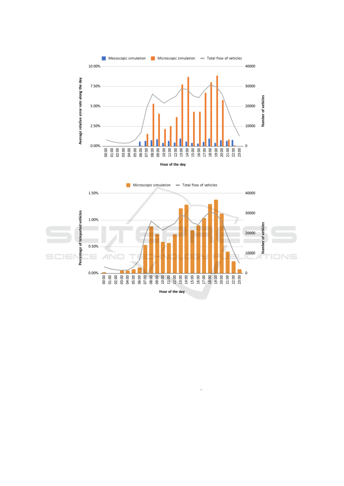
Figure 12: Hourly simulation errors along a day.
Figure 13: Hourly teleports along the day with a microscopic simulation.
current traffic model by considering additional data
sources. For example, traffic data captured by the an-
nual stations (mobile traffic-detection devices) could
be added as an input to the model; the difficulty with
this type of input data is that it is quite sparse, as each
mobile device stays in the same location measuring
data only during a few days, and therefore applying
any machine learning procedure to model traffic using
these data is challenging. Besides, we would like to
sophisticate the way that special events can be defined
and provided by the user who wants to perform a sim-
ulation, which is currently based on the application of
extra weights over the expected traffic. It would also
be relevant to allow the user to specify hypothetical
traffic situations (e.g., restrictions for the circulation
of certain types of vehicles in the downtown of a city)
to see the impact on traffic (what-if analysis).
ACKNOWLEDGEMENTS
This work has been supported by the project
TIN2016-78011-C4-3-R (AEI/FEDER, UE), by the
TRAFAIR project (2017-EU-IA-0167), co-financed
by the Connecting Europe Facility of the European
Union, and the Government of Aragon (Group Refer-
ence T64 20R, COSMOS research group). The con-
tents of this publication are the sole responsibility of
its authors and do not necessarily reflect the opinion
of the European Union. We thank the City Council of
Zaragoza (Ayuntamiento de Zaragoza) for providing
WEBIST 2020 - 16th International Conference on Web Information Systems and Technologies
126

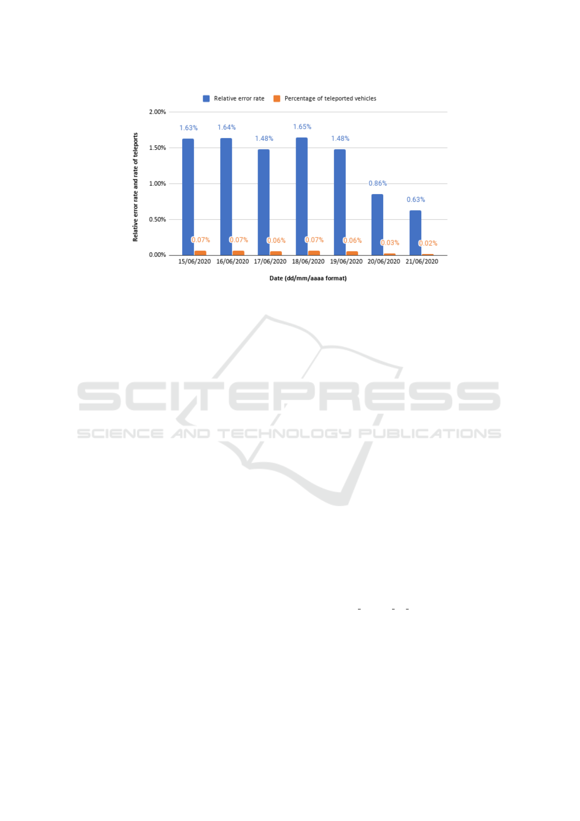
Figure 14: Relative error rate and percentage of teleported vehicles along a week using mesoscopic simulations.
us historical traffic sensor data on a regular basis. The
maps of the cities used in the experiments are derived
from data obtained from OpenStreetMap.
REFERENCES
Aiken, L. S., West, S. G., Pitts, S. C., Baraldi, A. N., and
Wurpts, I. C. (2012). Multiple Linear Regression,
chapter 18. American Cancer Society.
Anastasi, G., Antonelli, M., Bechini, A., Brienza, S.,
D’Andrea, E., Guglielmo, D. D., Ducange, P.,
Lazzerini, B., Marcelloni, F., and Segatori, A. (2013).
Urban and social sensing for sustainable mobility in
smart cities. In 2013 Sustainable Internet and ICT for
Sustainability (SustainIT). IEEE.
Anenberg, S. C., Henze, D. K., Tinney, V., Kinney, P. L.,
Raich, W., Fann, N., Malley, C. S., Roman, H., Lam-
sal, L., Duncan, B., Martin, R. V., van Donkelaar,
A., Brauer, M., Doherty, R., Jonson, J. E., Davila, Y.,
Sudo, K., and Kuylenstierna, J. C. (2018). Estimates
of the global burden of ambient PM2.5, ozone, and
NO2 on asthma incidence and emergency room visits.
Environmental Health Perspectives, 126(10):107004–
1–107004–14.
Behrisch, M., Bieker, L., Erdmann, J., and Krajzewicz, D.
(2011). SUMO – Simulation of Urban MObility: An
overview. In Third International Conference on Ad-
vances in System Simulation (SIMUL), pages 55–60.
IARIA.
Camp, T., Boleng, J., and Davies, V. (2002). A survey of
mobility models for ad hoc network research. Wireless
Communications and Mobile Computing, 2(5):483–
502.
Chowdhury, D., Santen, L., and Schadschneider, A. (2000).
Statistical physics of vehicular traffic and some related
systems. Physics Reports, 329(4):199–329.
Curtis, L., Rea, W., Smith-Willis, P., Fenyves, E., and Pan,
Y. (2006). Adverse health effects of outdoor air pollu-
tants. Environment International, 32(6):815–830.
Dickson, I. (2020). Before and after COVID-19: Europe’s
traffic congestion mapped. HERE Technologies, http
s://360.here.com/covid-19-impact-traffic-congestion
[Accessed: August 24, 2020].
Djahel, S., Doolan, R., Muntean, G.-M., and Murphy, J.
(2015). A communications-oriented perspective on
Traffic Management Systems for smart cities: Chal-
lenges and innovative approaches. IEEE Communica-
tions Surveys & Tutorials, 17(1):125–151.
Eissfeldt, N. G. (2004). Vehicle-based modelling of traf-
fic – Theory and application to environmental impact
modelling. PhD thesis, Universit
¨
at zu K
¨
oln. http:
//kups.ub.uni-koeln.de/id/eprint/1274 [Accessed:
August 24, 2020].
Erdmann, J. (2012). Online-kalibrierung einer mikroskopis-
chen verkehrssimulation. In ViMOS 2012. https:
//elib.dlr.de/79428 [Accessed: August 24, 2020,
2020].
German Aerospace Center (DLR), Institute of Transporta-
tion Systems (2019a). SUMO – simulation/meso.
https://sumo.dlr.de/docs/Simulation/Meso.html,
[Accessed: August 24, 2020].
German Aerospace Center (DLR), Institute of Transporta-
tion Systems (2019b). SUMO – simulation/why vehi-
cles are teleporting. https://sumo.dlr.de/docs/Simul
ation/Why
Vehicles are teleporting.html, [Accessed:
August 24, 2020].
German Aerospace Center (DLR), Institute of Transporta-
tion Systems (2020a). SUMO – NETCONVERT.
https://sumo.dlr.de/docs/NETCONVERT.html, [Ac-
cessed: August 24, 2020].
German Aerospace Center (DLR), Institute of Transporta-
tion Systems (2020b). SUMO – netedit. https:
//sumo.dlr.de/docs/NETEDIT.html, [Accessed: Au-
gust 24, 2020].
Traffic Flow Modelling for Pollution Awareness: The TRAFAIR Experience in the City of Zaragoza
127

German Aerospace Center (DLR), Institute of Transporta-
tion Systems (2020c). SUMO – simulation/calibrator.
https://sumo.dlr.de/docs/Simulation/Calibrator.html,
[Accessed: August 24, 2020].
Google (2020). Google Maps. http://maps.google.com/.
Accessed: August 24, 2020.
H
¨
arri, J., Filali, F., and Bonnet, C. (2009). Mobility models
for vehicular ad hoc networks: a survey and taxon-
omy. IEEE Communications Surveys and Tutorials,
11(4):19–41.
H
¨
arri, J., Filali, F., Bonnet, C., and Fiore, M. (2006). Vanet-
MobiSim: Generating realistic mobility patterns for
VANETs. In Third International Workshop on Vehic-
ular Ad Hoc Networks (VANET), pages 96–97, New
York, NY, USA. ACM.
H
¨
arri, J., Fiore, M., Filali, F., and Bonnet, C. (2011). Vehic-
ular mobility simulation with VanetMobiSim. SIMU-
LATION, 87(4):275–300.
Hu, Y., Barbour, W., Samaranayake, S., and Work, D.
(2020). Impacts of Covid-19 mode shift on road traf-
fic. arXiv:2005.01610.
Ilarri, S., Delot, T., and Trillo-Lado, R. (2015). A data
management perspective on vehicular networks. IEEE
Communications Surveys and Tutorials, 17(4):2420–
2460.
Krajzewicz, D., Hertkorn, G., R
¨
ossel, C., and Wagner, P.
(2002). SUMO (Simulation of Urban MObility) – an
open-source traffic simulation. In Fourth Middle East
Symposium on Simulation and Modelling (MESM),
pages 183–187.
Krauß, S. (1998). Microscopic Modeling of Traffic Flow:
Investigation of Collision Free Vehicle Dynamics.
PhD thesis, Universit
¨
at zu K
¨
oln. http://e-archive.in
formatik.uni-koeln.de/id/eprint/319 [Accessed: Au-
gust 24, 2020].
La
˜
na, I., Ser, J. D., Padr
´
o, A., V
´
elez, M., and Casanova-
Mateo, C. (2016). The role of local urban traffic and
meteorological conditions in air pollution: A data-
based case study in Madrid, Spain. Atmospheric En-
vironment, 145:424–438.
Lopez, P. A., Behrisch, M., Bieker-Walz, L., Erdmann,
J., Fl
¨
otter
¨
od, Y., Hilbrich, R., L
¨
ucken, L., Rummel,
J., Wagner, P., and Wiessner, E. (2018). Micro-
scopic traffic simulation using SUMO. In 21st In-
ternational Conference on Intelligent Transportation
Systems (ITSC), pages 2575–2582.
Mayer, H. (1999). Air pollution in cities. Atmospheric En-
vironment, 33(24-25):4029–4037.
OpenSim Ltd. (2000). OMNeT++. https://omnetpp.org/.
Accessed: August 24, 2020.
OpenStreetMap Foundation (OSMF) (2004). Open-
StreetMap. https://www.openstreetmap.org, [Ac-
cessed: August 24, 2020].
Po, L., Rollo, F., Viqueira, J. R. R., Lado, R. T., Bigi,
A., L
´
opez, J. C., Paolucci, M., and Nesi, P. (2019).
TRAFAIR: Understanding Traffic Flow to Improve
Air Quality. In 2019 IEEE International Smart Cities
Conference (ISC2 2019), pages 36–43.
PostGIS Team (2001). PostGIS. https://postgis.net/. Ac-
cessed: August 24, 2020.
QGIS Development Team (2004). QGIS – a free and open
source geographic information system. https://www.
qgis.org/. Accessed: August 24, 2020.
Samet, J. M. (2007). Traffic, air pollution, and health. In-
halation Toxicology, 19(12):1021–1027.
Sharif, A., Li, J., Khalil, M., Kumar, R., Sharif, M. I., and
Sharif, A. (2017). Internet of Things — smart traffic
management system for smart cities using Big Data
analytics. In 14th International Computer Conference
on Wavelet Active Media Technology and Informa-
tion Processing (ICCWAMTIP 2017), pages 281–284.
IEEE.
Sommer, C. (2006). VEINS (Vehicles in Network Simula-
tor). http://veins.car2x.org/. Accessed: August 24,
2020.
Sommer, C., German, R., and Dressler, F. (2011). Bidi-
rectionally coupled network and road traffic simula-
tion for improved IVC analysis. IEEE Transactions
on Mobile Computing (TMC), 10(1):3–15.
The PostgreSQL Global Development Group (1996). Post-
greSQL. https://www.postgresql.org/. Accessed:
August 24, 2020.
TRAFAIR Team (2018). Website of TRAFAIR – under-
standing traffic flows to improve air quality. https:
//trafair.eu/. Accessed: August 24, 2020. INEA CEF-
TELECOM Project co-funded by European Union.
Grant Agreement n. INEA/CEF/ICT/A2017/1566782
of August 7, 2018.
Trillo, R., Ilarri, S., and Mena, E. (2007). Comparison and
performance evaluation of mobile agent platforms. In
Third International Conference on Autonomic and Au-
tonomous Systems (ICAS), pages 41–46. IEEE Com-
puter Society.
Urra, O. and Ilarri, S. (2016). Cognitive Vehicular Net-
works, chapter 10 “MAVSIM: Testing VANET Ap-
plications Based on Mobile Agents”, pages 199–224.
CRC Press – Taylor & Francis Group. Print ISBN:
978-1-4987-2191-2, eBook ISBN: 978-1-4987-2192-
9.
Worldsensing (2018). Traffic Flow Management in
Zaragoza City – Success Story. https://www.worl
dsensing.com/wp-content/uploads/2018/01/v1 Plant
illa Success Story Bitcarrier Traffic-Flow-Manage
ment-in-Zaragoza-City.pdf, [Accessed: August 24,
2020].
Worldsensing (2020). Bitcarrier – The real-time Traffic
Flow Monitoring System. https://www.worldsensi
ng.com/product/bitcarrier/, [Accessed: August 24,
2020].
WEBIST 2020 - 16th International Conference on Web Information Systems and Technologies
128