
Large-scale Retrieval of Bayesian Machine Learning Models
for Time Series Data via Gaussian Processes
Fabian Berns
1
and Christian Beecks
1,2
1
Department of Computer Science, University of M
¨
unster, Germany
2
Fraunhofer Institute for Applied Information Technology FIT, Sankt Augustin, Germany
christian.beecks@fit.fraunhofer.de
Keywords:
Bayesian Machine Learning, Gaussian Process, Data Modeling, Knowledge Discovery.
Abstract:
Gaussian Process Models (GPMs) are widely regarded as a prominent tool for learning statistical data models
that enable timeseries interpolation, regression, and classification. These models are frequently instantiated
by a Gaussian Process with a zero-mean function and a radial basis covariance function. While these default
instantiations yield acceptable analytical quality in terms of model accuracy, GPM retrieval algorithms au-
tomatically search for an application-specific model fitting a particular dataset. State-of-the-art methods for
automatic retrieval of GPMs are searching the space of possible models in a rather intricate way and thus
result in super-quadratic computation time complexity for model selection and evaluation. Since these proper-
ties only enable processing small datasets with low statistical versatility, we propose the Timeseries Automatic
GPM Retrieval (TAGR) algorithm for efficient retrieval of large-scale GPMs. The resulting model is composed
of independent statistical representations for non-overlapping segments of the given data and reduces compu-
tation time by orders of magnitude. Our performance analysis indicates that our proposal is able to outperform
state-of-the-art algorithms for automatic GPM retrieval with respect to the qualities of efficiency, scalability,
and accuracy.
1 INTRODUCTION
Applying Gaussian Process Models (GPMs) for inter-
polation (Roberts et al., 2013; Li and Marlin, 2016),
regression (Titsias, 2009; Duvenaud et al., 2013), and
classification (Li and Marlin, 2016; Hensman et al.,
2013) of timeseries necessitates to instantiate the un-
derlying Gaussian Process by a covariance function
and a mean function. While the latter is typically in-
stantiated by a constant, zero-mean function, the co-
variance function is modelled either by (i) a general-
purpose kernel (Wilson and Adams, 2013), (ii) a
domain-specific kernel that is individually tailored to
a specific application by a domain expert (Wilson and
Adams, 2013; Abrahamsen and Petter, 1997; Ras-
mussen and Williams, 2006), or (iii) a composite ker-
nel that is computed automatically by means of a
GPM retrieval process (Duvenaud et al., 2013; Lloyd
et al., 2014) in order to decompose the statistical
characteristics underlying the data into multiple sub-
models. Although the first option (i) produces GPMs
of sufficiently high model accuracy, both (ii) and (iii)
encapsulate data’s peculiarities and versatilities in a
more detailed manner. Making use of domain-specific
kernels requires laborious fine-tuning and extensive
expert knowledge. Employing an automatic, domain-
agnostic GPM retrieval process on the other hand pro-
duces expressive composite kernels without requiring
any human interference.
State-of-the-art automatic GPM retrieval algo-
rithms, such as Compositional Kernel Search (CKS)
(Duvenaud et al., 2013), Automatic Bayesian Covari-
ance Discovery (ABCD) (Lloyd et al., 2014; Stein-
ruecken et al., 2019) and Scalable Kernel Compo-
sition (SKC) (Kim and Teh, 2018), apply an open-
ended greedy search in the space of all feasible com-
posite covariance functions in order to determine an
optimal, e.g. in terms of maximum likelihood, in-
stantiation of the underlying Gaussian Process. The
resulting inextricable GPM needs to account for all
different kinds of statistical peculiarities of the un-
derlying data and thus lacks expressiveness especially
with regards to local phenomena. Additionally, evalu-
ating a GPM by usual measures such as the likelihood
(Malkomes et al., 2016) function entails calculations
of cubic computation time complexity, which limits
Berns, F. and Beecks, C.
Large-scale Retrieval of Bayesian Machine Learning Models for Time Series Data via Gaussian Processes.
DOI: 10.5220/0010109700710080
In Proceedings of the 12th International Joint Conference on Knowledge Discovery, Knowledge Engineering and Knowledge Management (IC3K 2020) - Volume 1: KDIR, pages 71-80
ISBN: 978-989-758-474-9
Copyright
c
2020 by SCITEPRESS – Science and Technology Publications, Lda. All rights reserved
71

the application of GPM retrieval algorithms to small-
to-moderate data collections (Kim and Teh, 2018).
In this paper, we aim to overcome the perfor-
mance limitations of state-of-the-art GPM retrieval al-
gorithms and propose the Timeseries Automatic GPM
Retrieval (TAGR) algorithm for large-scale statistical
data modeling based on Gaussian Processes. We aim
to limit the algorithm’s overall complexity by concur-
rently initiating multiple kernel searches on dynami-
cally partitioned data (cf. Berns and Beecks, 2020b,a;
Berns et al., 2019). In this way, TAGR describes
large-scale datasets by means of a concatenation of
independent sub-models. Our approach is able to out-
perform existing kernel search methods in terms of
expressiveness, while reducing execution time by a
factor of up to 500.
The paper is structured as follows. Section 2
presents related work and background information.
Section 3 introduces large-scale GPMs, while Section
4 proposes the corresponding TAGR algorithm. Its
performance and explanatory capacity are evaluated
in Section 5. We conclude our paper with an outlook
on future work in Section 6.
2 BACKGROUND AND RELATED
WORK
2.1 Gaussian Process
A Gaussian Process (Rasmussen and Williams,
2006) is a stochastic process over random variables
{ f (x) | x ∈ X }, indexed by a set X , where every sub-
set of random variables follows a multivariate normal
distribution. The distribution of a Gaussian Process is
the joint distribution of all of these random variables
and it is thus a probability distribution over the space
of functions { f | f : X → R}. A Gaussian Process is
formalized as follows:
f (·) ∼ GP
m(·), k(·, ·)
(1)
where the mean function m : X → R and the co-
variance function k : X × X → R are defined ∀x ∈ X
as follows:
m(x) = E [ f (x)] (2)
k(x, x
0
) = E
( f (x) − m(x)) ·
f (x
0
) − m(x
0
)
(3)
Given a finite dataset D = {X,Y } with X =
{x
i
| x
i
∈ X ∧ 1 ≤ i ≤ n} representing the underlying
input data (such as timestamps) and Y = { f (x
i
) | x
i
∈
X } representing the target data values, such as sen-
sor values or other complex measurements, the mean
and covariance functions are determined by maxi-
mizing the log marginal likelihood (Rasmussen and
Williams, 2006) of the Gaussian Process, which is de-
fined as follows:
L(m, k, θ | D) = −
1
2
·
(y − µ)
T
K
−1
(y − µ)+
logdet(K) +nlog(2π)] (4)
As can be seen in Equation 4, the marginaliza-
tion of a Gaussian Process for a given dataset D of
n records results in a finite data vector y ∈ R
n
, a mean
vector µ ∈ R
n
, and a covariance matrix K ∈ R
n×n
which are defined as y[i] = f (x
i
), µ[i] = m(x
i
), and
K[i, j] = k(x
i
, x
j
) for 1 ≤ i, j ≤ n, respectively. We use
the short-hand notation GP
θ
to denote a GPM whose
underlying mean function m and covariance function
k are parameterized via hyperparameters θ (cf. Cheng
and Boots, 2017; Csat
´
o and Opper, 2000).
While the covariance function is frequently used
as major data modeling entity it often lacks in de-
scribing individual statistical behaviors in a structured
way. To this end, Duvenaud et al. (2013) propose
to approximate and structure the covariance function
via multiple compositional kernel expressions in or-
der to obtain the resulting compositional kernel-based
covariance function. The corresponding algorithms
for automatically retrieving a GPM given an arbitrary
dataset D are summarized in the following section.
2.2 Retrieval Algorithms
GPM retrieval algorithms, such as CKS (Duvenaud
et al., 2013), ABCD (Lloyd et al., 2014; Steinruecken
et al., 2019), and SKC (Kim and Teh, 2018), aim to
discover the statistical structure of a dataset D by de-
termining an optimal covariance function k
1
. For this
purpose, the mean function of the Gaussian Process
is commonly instantiated by a constant zero function
(Duvenaud et al., 2013; Rasmussen and Williams,
2006), so as to correspond to an additional data nor-
malization step. The covariance function is algorith-
mically composed via operators implementing addi-
tion and multiplication among different (composed)
base kernels b ∈ B. Prominent base kernels include
the linear kernel, radial basis function kernel, and pe-
riodic kernel, which are able to capture for instance
smooth, jagged, and periodic behavior (Duvenaud
et al., 2013).
The algorithms mentioned above apply an open-
ended, greedy search in the space of all feasible ker-
nel combinations in order to progressively compute a
GPM fitting the entire dataset D, respectively Y ∈ D.
1
In (Berns and Beecks, 2020a), we detail the problem
and definition of automatic GPM retrieval.
KDIR 2020 - 12th International Conference on Knowledge Discovery and Information Retrieval
72

The CKS algorithm (Duvenaud et al., 2013) follows
a simple iterative procedure, called Basic Kernel Ex-
pansion Strategy (BES), which aims to improve the
best kernel expressions k retrieved in one iteration
over the course of the next one. Therefore, this strat-
egy produces a set of candidate kernel expressions C
k
based on k (Duvenaud et al., 2013):
C
k
=
{
k b | b ∈ B ∧ ∈ {+, ×}
}
(5)
Starting with a set of base kernels B, the candi-
dates of every following iteration are generated via
expanding upon the best candidate of the previous it-
eration. Moreover, a new candidate is also generated
for every replacement of a base kernel b with another
one b
0
. ABCD extends that grammar with regards to
a sigmoid change point operator | , in order to locally
restrict the effect of kernel expressions (Lloyd et al.,
2014; Steinruecken et al., 2019):
C
k
=
{
k b | b ∈ B ∧ ∈ {+, ×, | }
}
(6)
The performance of those given automatic GPM
retrieval algorithms is impeded by two major bottle-
necks. Evaluating every expansion of every subex-
pression poses one of these bottlenecks. Thus, reduc-
ing the set of candidates per iteration in order to cover
just the most promising candidates improves on the
performance of the respective algorithms, presumably
without affecting model quality. Moreover, assess-
ing model quality in terms of log marginal likelihood
epitomizes another bottleneck of current algorithms,
which is intrinsic to the framework of Gaussian Pro-
cesses itself (Hensman et al., 2013). The cubic run-
time complexity of that basic measure inhibits analy-
sis of large-scale datasets (cf. Kim and Teh, 2018).
Kim and Teh (2018) present SKC as a way to
overcome at least the latter one of those bottlenecks.
The algorithm improves the efficiency of the ker-
nel search process by accelerating CKS using the
Nystr
¨
om method (cf. Williams and Seeger, 2000) for
global approximations (Kim and Teh, 2018). This
low-rank matrix approximations constructs an ap-
proximate covariance matrix by means of a small sub-
set of the given data (cf. Gittens and Mahoney, 2016)
and allows to retrieve GPMs for datasets of up to
100,000 records in a reasonable amount of time ac-
cording to Kim and Teh (2018).
To summarize, state-of-the-art GPM retrieval al-
gorithms are not suited for the analysis of large-scale
datasets beyond 100,000 records due to their cubic
computation time complexity as well as due to their
large candidate sets, which need to be evaluated dur-
ing the search procedure (cf. Kim and Teh, 2018).
3 LARGE-SCALE GAUSSIAN
PROCESS MODELS
In this section, we propose the structural design of
large-scale GPMs. It is designed to reduce computa-
tional complexity of GPM evaluations as well as to
mitigate the amount of kernel expression candidates,
which need to be evaluated as part of the respective re-
trieval algorithm. Since these two issues are the main
bottlenecks of current GPM retrieval algorithms, re-
spective solution strategies are separately covered in
the following two subsections.
3.1 Reduction of Computational
Complexity
Liu et al. (2020) as well as Rivera and Burnaev
(2017) highlight local approximations as a key pos-
sibility to reduce complexity of common GPM eval-
uations based on likelihood measures. Instead of in-
fering an approximate GPM based on a data subset
(cf. global approximations), they construct a holis-
tic GPM from locally-specialized models trained on
non-overlapping segments of the data. Thus, the co-
variance matrix of the holistic GPM is composed of
the respective matrices of its local sub-models (Liu
et al., 2020). This divide-&-conquer approach accel-
erates calculation of log marginal likelihood, since the
resulting covariance matrix is a block diagonal matrix
(Rivera and Burnaev, 2017), whose inverse and deter-
minant can be computed efficiently (Park and Apley,
2018). Rivera and Burnaev (2017) emphasize that lo-
cal approximations allow to ”model rapidly-varying
functions with small correlations” in contrast to low-
rank matrix approximations.
Embedding the concept of local approximations
into GPM retrieval algorithms requires a globally
partitioning covariance function. While in principle
change point operators facilitate a global data par-
titioning, their nature of fading kernel expressions
into one another (Lloyd et al., 2014; Steinruecken
et al., 2019) does neither produce clear boundaries be-
tween sub-models nor enables independence of these
models. Therefore, we adapt the given notion of a
change point operator to utilize indicator functions
(Iliev et al., 2017) instead of sigmoid functions (cf.
Steinruecken et al., 2019) to separate kernel expres-
sions. This leads us to the definition of a parti-
tioning covariance function K for large-scale GPMs
GP
θ
(0, K ):
K (x, x
0
| {k
b
}
m
b=1
, {τ
b
}
m
b=0
) =
m
∑
b=1
k
b
(x, x
0
) · 1
{τ
b−1
<x≤τ
b
}
(x) · 1
{τ
b−1
<x
0
≤τ
b
}
(x
0
) (7)
Large-scale Retrieval of Bayesian Machine Learning Models for Time Series Data via Gaussian Processes
73

The parameter m ∈ N defines the number of sub-
models k
b
: X ×X → R, where each sub-model k
b
can
be thought of as a local covariance function model-
ing the restricted domain [τ
b−1
, τ
b
] ⊆ X . In this way,
each sub-model k
b
is only responsible for a certain
coherent fraction of the data, which is delimited by
the change points τ
b−1
and τ
b
. The specific change
points τ
0
= x
1
and τ
m
= x
n
denote the start and end of
the data set D. The usage of indicator functions (thus
having disjoint data segments) produces a block diag-
onal covariance matrix (cf. Low et al., 2015), which
facilitates independently searching the most likely lo-
cal kernel expression (i.e. sub-model) per data seg-
ment.
In order to mathematically show the implication
of aforementioned independence, we have to inves-
tigate the internal structure of the corresponding log
marginal likelihood function L(m, k, θ | D). To this
end, we assume the inherent covariance matrix K ∈
R
n×n
(cf. Equation 4) to be a block diagonal matrix.
That is, it holds that K = diag(K
1
, ..., K
m
), where each
matrix K
b
∈ R
n
b
×n
b
for 1 ≤ b ≤ m is of individual ar-
bitrary size n
b
∈ N such that
∑
b
n
b
= n. Furthermore,
let (I
1
, ..., I
m
) denote the partitioning of index set
{1, ..., n} ⊆ N according to the given blocks, i.e. for a
submatrix of K over index set I
b
the following holds:
K
I
b
,I
b
= K
b
∀b ∈ [1, m]. Given this notation, one can
show (i) that the quadratic form (y − µ)
T
K
−1
(y − µ)
of the log marginal likelihood function L(m, k, θ | D)
is equivalent to
∑
m
b=1
( ˜y
b
− ˜µ
b
)
T
K
−1
b
( ˜y
b
− ˜µ
b
), where
˜y
b
= (y
i
)
i∈I
b
∈ R
n
b
and ˜µ
b
= (µ
i
)
i∈I
b
∈ R
n
b
are de-
fined according to the block diagonal structure and
(ii) that the logarithmic determinant can be decom-
posed as follows: log det(K) = log
∏
m
b=1
det(K
b
) =
∑
m
b=1
logdet(K
b
). By making use of the aforemen-
tioned algebraic simplifications, we can simplify the
calculation of the log marginal likelihood function as
shown below:
L(m, k, θ | D)
= −
1
2
·
(y − µ)
T
K
−1
(y − µ) + log det(K) + n log(2π)
= −
1
2
·
"
m
∑
b=1
( ˜y
b
− ˜µ
b
)
T
K
−1
b
( ˜y
b
− ˜µ
b
)
+
n
∑
b=1
logdet(K
b
) +
m
∑
b=1
n
b
· log(2π)
#
=
m
∑
b=1
−
1
2
·
h
( ˜y
b
− ˜µ
b
)
T
K
−1
b
( ˜y
b
− ˜µ
b
)
+ log det(K
b
) + n
b
log(2π)
i
=
m
∑
b=1
L(m, k
b
, θ | D
b
)
(8)
As shown above, the equivalence L(m, k, θ | D) =
∑
m
b=1
L(m, k
b
, θ | D
b
) affects the computation of a
large-scale GPM by means of K for a given data
set D and its non-overlapping partitions D
b
. Instead
of jointly optimizing a holistic statistical model fit-
ting the entire data set D, we are able to indepen-
dently optimize individual sub-models k
b
. This will
not only increase the expressiveness of the overall
GPM, but also reduce the computation time required
for calculating such a model. Moreover, by splitting a
GPM into smaller parts, we enable a large-scale GPM
to be computed by means of the divide-&-conquer
paradigm. Before we investigate the proposed algo-
rithmic solution, we continue with describing strate-
gies for efficiently reducing the size of candidate sets
for sub-models k
b
.
3.2 Expansion Strategies
In contrast to the previous section, where we have
shown how to reduce the complexity of evaluating a
single GPM via a divide-&-conquer-based approach,
we investigate measures to reduce the amount of
to-be-evaluated candidates per sub-model covariance
function k
b
in the remainder of this section. Equation
5 and 6 illustrate the state-of-the-art strategy used by
CKS (Duvenaud et al., 2013), SKC (Kim and Teh,
2018) and ABCD (Lloyd et al., 2014). While this
strategy allows to exhaustively search the space of
possible kernel expressions for the most appropriate
one, it entails to evaluate a lot of inferior candidates
as a by-product. Since the sub-models k
b
of K (cf.
Equation 7) are designed to represent independent and
inseparable behavioral patterns, introducing further
change points on that layer of the covariance function
would contradict the atomicity assumption of every
sub-model k
b
. Furthermore, by focusing on compos-
ite covariance functions which are only derived by ad-
ditions and multiplications of base kernels, the num-
ber of candidate models can be further reduced.
Although state-of-the-art algorithms consider
every possible kernel expansion regardless of their
structure up to a certain depth (cf. Subsection
2.2), they retroactively enforce a hierarchy, i.e., the
so-called Sum-of-Products (SoP) hierarchy (Duve-
naud et al., 2013) (cf. Equation 9), among additive
operators and multiplicative operators. Thus, these
algorithms structure the resulting kernel expressions
in order to foster comprehensibility in hindsight. We
incorporate that SoP hierarchy into our kernel expan-
sion strategy to prohibit functionally redundant com-
posite kernel expressions, which result from different
expressions producing the same SoP form, and define
KDIR 2020 - 12th International Conference on Knowledge Discovery and Information Retrieval
74

the set of SoP kernel expressions S as follows:
S =
(
s
∑
i=1
p
∏
j=1
b
i j
|b
i j
∈ B
)
(9)
Based on the mathematically formalization of the
SoP form given in the equation above, we propose the
new SoP Kernel Expansion Strategy (SES) by means
of the following candidate set:
C
k
=
{
k b| b ∈ B ∧ ∈ {+, ×} ∧ (k b) ∈ S
}
(10)
This candidate set ensures, that the resulting ker-
nel expression complies with the SoP form. As with
state-of-the-art algorithms, base kernels are consid-
ered as initial candidates of this strategy.
Orthogonal to the described improvement on ker-
nel expansion strategies, we assess the tactic of base
kernel replacement as ineffectual from a theoreti-
cal perspective, as it contradicts the greedy search
(Resende and Ribeiro, 2016) propagated by authors
of state-of-the-art methods (cf. Steinruecken et al.,
2019). Therefore, we will separately analyze the ef-
fects of this replacement tactic on GPM retrieval in
Section 5.
To sum up, our structural design for large-scale
GPMs encompasses two solutions for the major bot-
tlenecks of GPM structures used by current state-of-
the-art algorithms. On the one hand, local approxi-
mations by means of an indicator change point opera-
tor reduce computational complexity by partitioning
a GPM into several locally-specialized sub-models.
On the other hand, reducing the amount of candidate
covariance functions per sub-model k
b
by employ-
ing SES mitigates evaluative calculations for inferior
models.
4 AUTOMATIC GPM RETRIEVAL
In this section, we propose the Timeseries Automatic
GPM Retrieval (TAGR) algorithm for efficient re-
trieval of large-scale GPMs. To this end, we make use
of the efficiency improvements, i.e. locally approxi-
mated covariance function and SoP Kernel Expansion
Strategy (SES), described in the previous section.
In order to limit the algorithm’s overall com-
plexity and to increase model locality, i.e. to cap-
ture and describe local evolving patterns underlying
the data, the TAGR algorithm initiates multiple lo-
cal kernel searches on dynamically partitioned data.
Subsequently, TAGR concatenates the resulting sub-
models, i.e. each independent composite kernel-
based covariance function k
b
, into a joint large-scale
GPM by means of K (cf. Equation 7) and a zero-
mean function.
Prior to the computation of these independent sub-
models, a global partitioning needs to be determined.
As the field of change point detection mechanisms
for partitioning a dataset via their target values y ∈
Y (Truong et al., 2020; Aminikhanghahi and Cook,
2017) is a well researched domain, we assume the
set of change points T to be one of the parameters
of TAGR. Besides T , the given dataset D = {X,Y }
(cf. Subsection 2.1) and complexity parameter c
max
,
restricting sub-model size, are given as parameters.
Algorithm 1 illustrates the TAGR algorithm.
Without loss of generality we initiate the sub-models
k
b
∈ K for every data partition D
b
bounded by change
points τ
b−1
and τ
b
via a white noise kernel k
W N
. The
set I encompasses the indices of all non-final sub-
models k
b
∈ K. The following while-loop is executed
until this set of indices is empty. During every iter-
ation the segment K
i
with the lowest model quality
by means of log marginal likelihood L is selected,
candidate kernel expressions C
K
i
for that segment are
found using the predefined kernel expansion strategy
and the best performing kernel expression k
?
is deter-
mined. If that kernel expression k
?
reaches maximum
complexity c
max
in terms of number of involved base
kernels or is equal to the previous best expression K
i
,
it is considered final and thus removed from I . Fi-
nally, a GPM utilizing a K -based concatenation of
sub-models k
b
∈ K and zero-mean is returned.
Algorithm 1: Timeseries Automatic GPM Retrieval.
function (D, c
max
, T )
K = {k
W N
}
|T |
i=1
I = {i}
|T |
i=1
while |I | > 0 do
i = argmin
i∈I
L(0, K
i
, θ |D
i
)
k
?
= arg max
k∈C
K
i
L(0, k, θ |D
i
)
if k
?
= K
i
∨ c(k
?
) ≥ c
max
then
I = I \ i
K
i
= k
?
return GP
θ
(0, K (·, ·|K, T ))
Since the given algorithm is designed to enable
large-scale applications of GPM retrieval, it may be
accelerated by optimizing multiple segments in paral-
lel. The practical capabilities of the TAGR algorithm,
both in an unparallelized as well as in a parallelized
manner, are evaluated in the following chapter. Al-
though we do not explicitly name that opportunity in
Algorithm 1, a preliminary GPM K may be returned
after every iteration of the while-loop making the al-
gorithm anytime capable.
Large-scale Retrieval of Bayesian Machine Learning Models for Time Series Data via Gaussian Processes
75

Table 1: Used Benchmark Datasets.
Dataset Name Size Dim.
1 Airline 144 2
2 Solar Irradiance 391 2
3 Mauna Loa 702 2
4 SML (Zamora-Mart
´
ınez et al., 2014) 4,137 24
2
5 Power Plant (T
¨
ufekci, 2014) 9,568 5
3
6 GEFCOM (Hong et al., 2014) 38,064 21
4
7 Jena Weather (Max Planck Institute for Biogeochemistry, 2019) 420,551 15
5
8 Household Energy (Hebrail and Berard, 2012) 2,075,259 9
6
5 EVALUATION
In this section, we investigate the performance of the
proposed TAGR algorithm in terms of efficiency and
accuracy. At first we are solely evaluating TAGR for
different configurations of complexity parameter c
max
and different kernel expansion strategies (cf. Sec-
tion 3.2) to investigate, how they affect model qual-
ity and runtime (cf. Section 5.2). Based on the
empirically proven best parameter configuration, we
compare the TAGR algorithm against the state-of-
the-art algorithms CKS, SKC and ABCD (cf. Sec-
tion 5.3). They serve as a baseline to assess effi-
ciency and accuracy of our proposed algorithm. Fi-
nally, TAGR’s scalability and runtime performance
on large-scale datasets is demonstrated in Section 5.4,
where we omit the evaluation of ABCD, SKC and
CKS due to their computation time complexity (Ras-
mussen and Williams, 2006), which impedes analyz-
ing larger datasets (Kim and Teh, 2018) (cf. Table 2).
5.1 Setup of Experiments
In order to ensure comparability with existing and
prospective algorithms, we base our experiments on
publicly available datasets, which were also used by
2
Dimension ”Carbon dioxide in ppm (room)” was used
as target Y .
3
Dimension ”electrical power output (P
E
)” was used as
target Y .
4
We chose one of the 20 utility zones (i.e. the first one)
as the informational content among zones may be consid-
ered equivalent Hong et al. (2014). Our thorough empirical
analysis indicated, that selecting this attribute over the other
zones hardly affected the results.
5
Dimension ”Air
Temperature” was used as target Y .
We are using the recognized intervall of this continuously
gathered dataset from 2009-01-01 to 2016-12-31 (cf. Chol-
let, 2018)
6
Dimension ”Global active power” was used as target
Y .
4.2 4.4
4.6
·10
−2
PELT
WindowBased
BottomUp
Binary
Model Error - MSE
460
480
500
Runtime - seconds
Figure 1: Impact of partitioning methods on average run-
time and average model error of the TAGR algorithm.
Duvenaud et al. (2013) and Lloyd et al. (2014) in
their papers proposing CKS and ABCD (datasets 1,
2, 3 in Table 1). Kim and Teh (2018) note that
datasets larger than a few thousand points are ”far
beyond the scope of [...] GP optimisation in CKS”
and consequently beyond the scope of ABCD as well.
Therefore, datasets 1 - 3 are rather small. Espe-
cially for scalability analysis, we include five addi-
tional datasets (datasets 4-8 in Table 1).
As we focus on time series data in this paper and
both algorithms CKS and ABCD have been evalu-
ated for strictly one-dimensional input X ⊆ R and out-
put data Y ⊆ R (Duvenaud et al., 2013; Lloyd et al.,
2014), we will design our evaluation procedure ac-
cordingly.
In order to reflect practical circumstances, all ex-
periments are executed on a 2019 Dell Laptop hav-
ing a 1.9 GHz CPU (4 cores / 8 threads) with 16
GB of RAM. All algorithms were implemented using
Python 3 and Tensorflow 2 (no GPU acceleration en-
abled). Since Duvenaud et al. (2013) and Lloyd et al.
(2014) used L just for optimizing models and Mean
Squared Error (MSE) for assessing model quality, we
will adopt that procedure as well. For every evalua-
tion, MSE reflects the five-fold cross-validated model
error.
KDIR 2020 - 12th International Conference on Knowledge Discovery and Information Retrieval
76
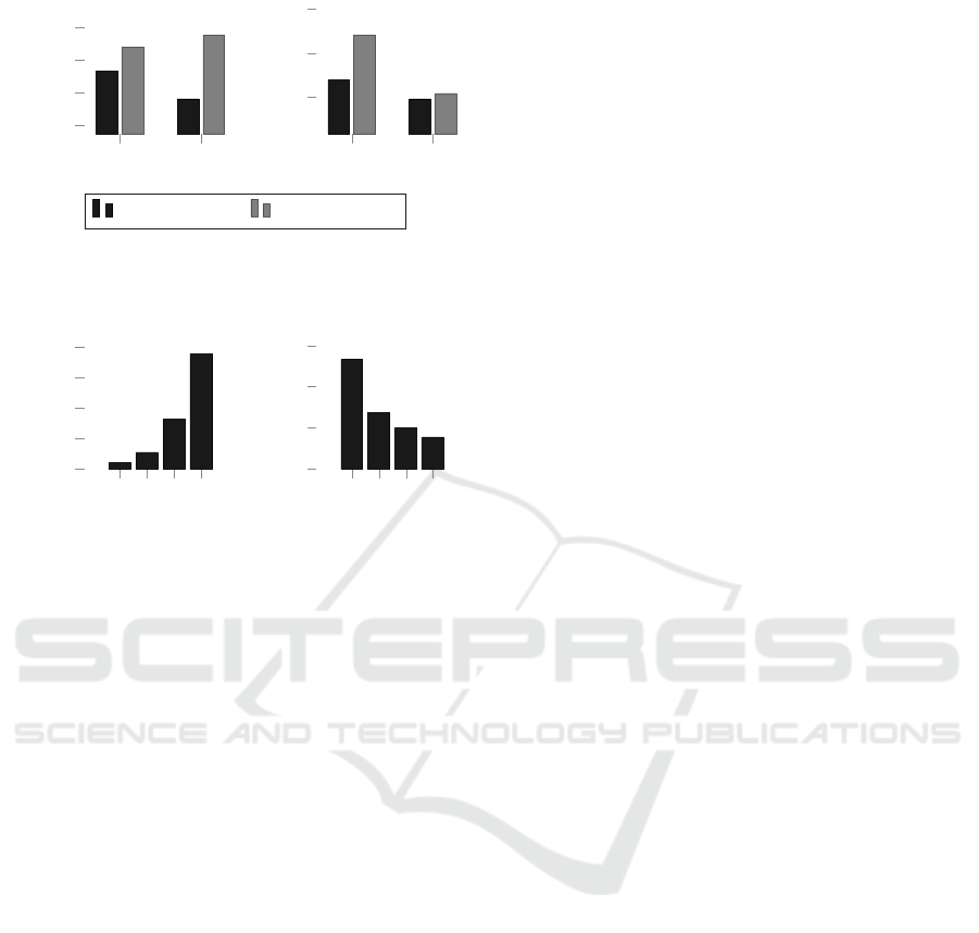
BES SES
40
60
80
100
Runtime - seconds
w/o replacement w/ replacement
BES SES
2
4
6
·10
−2
Model Error - MSE
Figure 2: Impact of kernel expansion strategy on average
runtime and average model error of the TAGR algorithm.
1 2 4 8
0
50
100
150
200
c
max
Runtime - seconds
1 2 4 8
0
2
4
6
·10
−2
c
max
Model Error - MSE
Figure 3: Impact of complexity parameter c
max
on average
runtime and average model error of the TAGR algorithm.
5.2 TAGR Configurations
In this first series of experiments, we evaluate the
influence of various change point detection mecha-
nisms to determine T , model complexity parameter
c
max
∈ [1, 2, 3, 4] and different kernel expansion strate-
gies (i.e. BES and SES) on both efficiency of the com-
putation, measured by runtime in seconds, and qual-
ity of the statistical model by MSE. We executed the
TAGR algorithm with all possible parameter configu-
rations on the datasets mentioned above (cf. Table 1).
All experiments of the first series execute the TAGR
algorithm in a non-parallel way. The results are sum-
marized in Figures 2 and 3.
At first, we evaluate, which standard change
point detection mechanism (cf. Truong et al., 2020;
Aminikhanghahi and Cook, 2017) to use in order to
determine the set of change points T as one of the
parameters of TAGR. To do so, we compare the four
mechanisms put forward by Truong et al. (2020) con-
sidering runtime performance and model error for ex-
ecuting TAGR utilizing the resulting change points.
Figure 1 illustrates the given performance indicators
averaged over all benchmark datasets and given pa-
rameter configurations of kernel expansion strategy
and complexity c
max
. Since Binary Segmentation of-
fers one of the lowest average model error and bene-
fits runtime the most, we choose this mean of change
point detection for further use of TAGR.
Figure 2 shows, how different kernel expansion
strategies impact average model error and average
runtime performance of the TAGR algorithm. In gen-
eral, BES is outperformed by SES and not using the
replacement tactic further improves on both of these
strategies. For most of the retrieved GPMs per bench-
mark dataset, the replacement tactic does not change
the resulting model and only increases runtime by in-
creasing the amount of candidate models. Still, some
GPM retrievals are negatively affected by employing
that tactic.
In addition to the different kernel expansion strate-
gies, we evaluated the complexity parameter c
max
.
While model error assessed by MSE is positively in-
fluenced by increasing complexity parameter c
max
,
the opposite holds true for runtime performance (cf.
Figure 3). Due to these results, we choose SES
and a model complexity of c
max
= 4 as default pa-
rameter configuration for the comparison of the pro-
posed TAGR algorithm with existing state-of-the-art
approaches. The chosen TAGR configuration does
not include the replacement tactic.
5.3 Comparison with State of the Art
In the second series of experiments, we compare the
performance in terms of model quality and runtime
of the TAGR algorithm to state-of-the-art algorithms.
In order to prevent interferences between paralleliz-
ability features and bare algorithmic qualities among
the evaluated competitors, all experiments of the sec-
ond series are executed in a non-parallel way. The
runtimes are summarized in Figure 4, while the cor-
responding detailed results are listed in Table 2.
As can be seen in Figure 4, the TAGR algorithm’s
divisive approach leads to a lower growth of runtime
in relation to the data size. This property comes es-
pecially handy for larger datasets. Considering for
example the dataset PowerPlant, the SKC algorithm
has a runtime of 9:19h (∼ 33,533 seconds), while the
TAGR algorithm only needs 0:01h (∼ 68 seconds)
to finish the corresponding computations. Hence,
our proposal is approximately up to 500 times as
fast as existing state-of-the-art solutions (SKC). This
huge improvement can be traced back to TAGR’s de-
sign, which not aims at retrieving one inextricable
large model, but one consisting of small, indepen-
dent partitions representing coherent fractions of the
data. Subsequently, model evaluations by means of
log marginal likelihood L or MSE are substantially
cheaper.
Besides ensuring better runtime properties of our
approach in comparison to CKS, ABCD and SKC, we
also show that TAGR produces statistical models by
Large-scale Retrieval of Bayesian Machine Learning Models for Time Series Data via Gaussian Processes
77
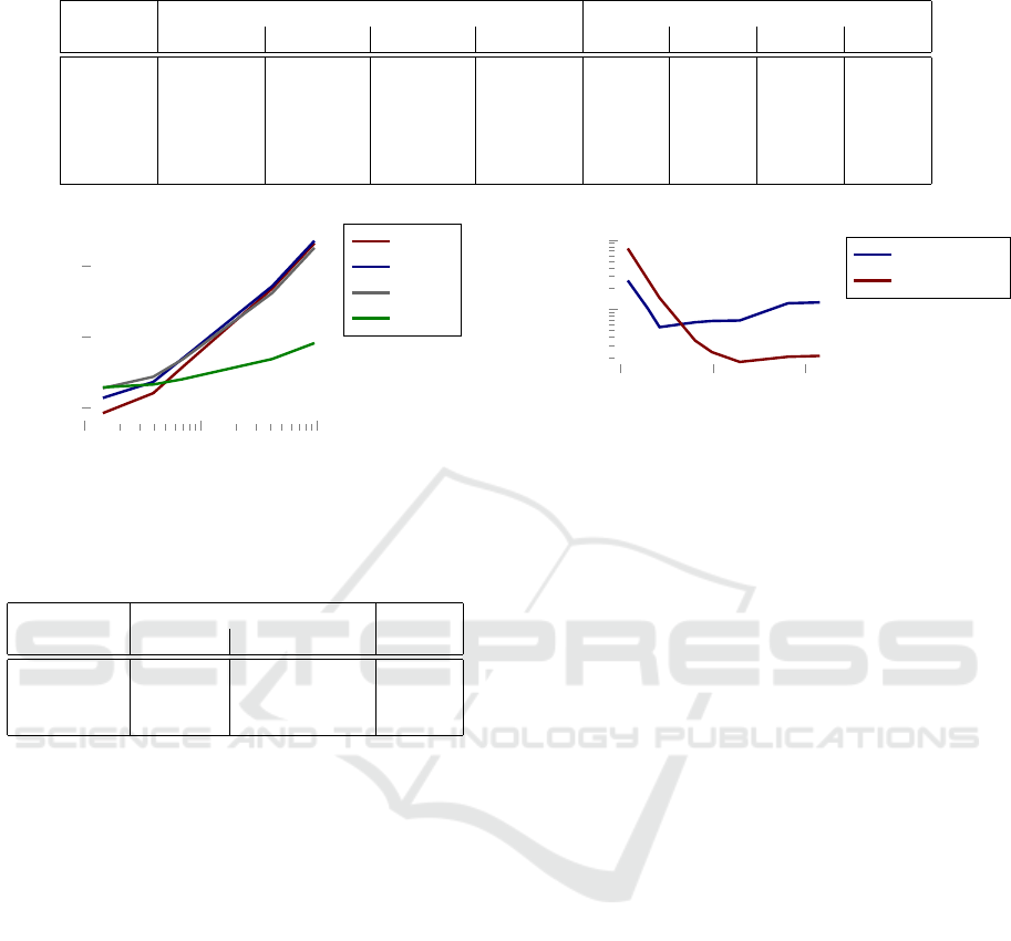
Table 2: Comparative evaluation results for state-of-the-art algorithms.
Runtime MSE
Dataset CKS ABCD SKC TAGR CKS ABCD SKC TAGR
Airline 00:00:01 00:00:02 00:00:04 00:00:04 0.1361 0.0981 0.1175 0.0269
Solar 00:00:03 00:00:06 00:00:08 00:00:05 0.0856 0.0897 0.0845 0.0769
Mauna 00:00:15 00:00:26 00:00:24 00:00:07 0.1525 0.1519 0.1724 0.0156
SML 00:39:05 00:45:52 00:29:18 00:00:25 0.1103 0.1103 0.2259 0.0112
Power 12:27:51 14:37:15 09:18:53 00:01:08 0.0726 0.0726 0.1772 0.0046
10
2
10
3
10
4
10
0
10
2
10
4
dataset size
Runtime - seconds
CKS
ABCD
SKC
TAGR
Figure 4: Runtime for different state-of-the-art algorithms
as a function of dataset size.
Table 3: Performance and Model Quality.
Runtime
Dataset Parallel Non-Parallel MSE
GEFCOM 0:03:44 0:13:09 0.0111
Jena 0:46:58 4:18:03 0.0109
Household 5:21:26 21:34:42 0.0024
means of kernel expressions of better quality. Table 2
illustrates the resulting model qualities per algorithm.
In general, TAGR delivers better results regarding ev-
ery dataset analyzed according to MSE measure.
5.4 Scalability of TAGR
The third and final series of experiments is only fo-
cused on evaluation of the TAGR algorithm. TAGR
clearly outperforms state-of-the-art algorithms in
terms of runtime, while still maintaining solid model
quality. Nevertheless, the largest dataset considered
comprises only approximately 10,000 records, which
is by no definition large-scale. Thus, we aim to show
the scalability features of our proposal in the remain-
der of this section, for which we employ the largest
three of the selected datasets (cf. Table 1), containing
up to two million records.
Table 3 presents the results of non-parallel and
parallel execution of the TAGR algorithm for the
given large-scale datasets. We executed it in a par-
allel as well as in a non-parallel fashion, to main-
tain comparability with given publications (cf. Lloyd
10
2
10
4
10
6
10
−2
10
−1
dataset size
runtime / dataset size
Non-Parallel
Parallel
Figure 5: Runtime per Data Record.
et al., 2014; Duvenaud et al., 2013; Kim and Teh,
2018; Steinruecken et al., 2019), while still show-
ing TAGR’s scalability features. As parallelization
of TAGR does not affect the resulting models, only
one qualitative measure concerning model accuracy
is given per analyzed dataset.
Figure 5 illustrates how the ratio between runtime
and dataset size evolves along absolute dataset size.
It shows that TAGR becomes more efficient facing in-
creasing dataset sizes. Beyond that, concurrent ex-
ecution of our proposed algorithms building blocks
reduces runtime compared to non-parallel execution.
Those mentioned advances do not obstruct the accu-
racy of the derived GPM as shown in Tables 2 and
3.
To sum up, we have shown which kind of param-
eter configuration of our algorithmic approach pro-
duces the most promising results regarding model
quality and performance. Based on that, we demon-
strated how our approach produces statistical data
models by means of Gaussian Processes of supe-
rior quality with regards to state-of-the-art algo-
rithms, while outperforming these algorithms con-
cerning runtime performance in general.
6 CONCLUSION
In this paper, we have investigated a new approach for
efficient, automatic GPM retrieval for large-scale time
series datasets. While state-of-the-art GPM retrieval
algorithms lack scalability (cf. Berns and Beecks,
2020b), we propose a new structural design for large-
scale GPMs. This design allows to get around the
KDIR 2020 - 12th International Conference on Knowledge Discovery and Information Retrieval
78

two major bottlenecks of current methods by using
a divisive approach to reduce effects of Gaussian Pro-
cesses’ cubic runtime complexity as well as employ-
ing a purposive strategy to generate fewer candidate
models.
Our performance evaluation has revealed that
GPMs resulting from the proposed TAGR algorithm
deliver similar model quality in comparison to those
models produced by state-of-the-art algorithms. In
addition, runtime of the retrieval process is reduced
significantly especially for larger time series, where
we achieve a speed-up factor of approximately 500
with regards to existing methods such as CKS, ABCD
and SKC.
As for future work, we consider global approxi-
mations an opportunity for further optimizing our ap-
proach. We therefore plan to address the opportuni-
ties of low-rank approximations such as the Nystr
¨
om
method (Hensman et al., 2013) in our future work.
In addition, we plan to develop GPM retrieval algo-
rithms for big data processing frameworks in order to
scale GPM retrieval to very large and even multidi-
mensional datasets.
REFERENCES
Abrahamsen and Petter (1997). A review of gaussian ran-
dom fields and correlation functions: Technical report
917.
Aminikhanghahi, S. and Cook, D. J. (2017). A survey
of methods for time series change point detection.
Knowl. Inf. Syst., 51(2):339–367.
Berns, F. and Beecks, C. (2020a). Automatic gaussian pro-
cess model retrieval for big data. In CIKM. ACM.
Berns, F. and Beecks, C. (2020b). Towards large-scale gaus-
sian process models for efficient bayesian machine
learning. In DATA, pages 275–282. SciTePress.
Berns, F., Schmidt, K. W., Grass, A., and Beecks, C. (2019).
A new approach for efficient structure discovery in iot.
In BigData, pages 4152–4156. IEEE.
Cheng, C. and Boots, B. (2017). Variational inference for
gaussian process models with linear complexity. In
NIPS, pages 5184–5194.
Chollet, F. (2018). Deep learning with Python. Manning
Publications Co, Shelter Island New York.
Csat
´
o, L. and Opper, M. (2000). Sparse representation for
gaussian process models. In NIPS, pages 444–450.
MIT Press.
Duvenaud, D., Lloyd, J. R., Grosse, R. B., Tenenbaum,
J. B., and Ghahramani, Z. (2013). Structure dis-
covery in nonparametric regression through composi-
tional kernel search. In ICML (3), volume 28 of JMLR
Workshop and Conference Proceedings, pages 1166–
1174. JMLR.org.
Gittens, A. and Mahoney, M. W. (2016). Revisiting the nys-
trom method for improved large-scale machine learn-
ing. J. Mach. Learn. Res., 17:117:1–117:65.
Hebrail, G. and Berard, A. (2012). Individual house-
hold electric power consumption data set.
https://archive.ics.uci.edu/ml/datasets/individual+
household+electric+power+consumption. Accessed:
09/01/2020.
Hensman, J., Fusi, N., and Lawrence, N. D. (2013). Gaus-
sian processes for big data. In UAI. AUAI Press.
Hong, T., Pinson, P., and Fan, S. (2014). Global energy
forecasting competition 2012. International Journal
of Forecasting, 30(2):357–363.
Iliev, A. I., Kyurkchiev, N., and Markov, S. (2017). On the
approximation of the step function by some sigmoid
functions. Math. Comput. Simul., 133:223–234.
Kim, H. and Teh, Y. W. (2018). Scaling up the automatic
statistician: Scalable structure discovery using gaus-
sian processes. In AISTATS, volume 84 of Proceed-
ings of Machine Learning Research, pages 575–584.
PMLR.
Li, S. C. and Marlin, B. M. (2016). A scalable end-to-end
gaussian process adapter for irregularly sampled time
series classification. In NIPS, pages 1804–1812.
Liu, H., Ong, Y., Shen, X., and Cai, J. (2020). When gaus-
sian process meets big data: A review of scalable gps.
IEEE Transactions on Neural Networks and Learning
Systems, pages 1–19.
Lloyd, J. R., Duvenaud, D., Grosse, R. B., Tenenbaum,
J. B., and Ghahramani, Z. (2014). Automatic con-
struction and natural-language description of nonpara-
metric regression models. In AAAI, pages 1242–1250.
AAAI Press.
Low, K. H., Yu, J., Chen, J., and Jaillet, P. (2015). Paral-
lel gaussian process regression for big data: Low-rank
representation meets markov approximation. In AAAI,
pages 2821–2827. AAAI Press.
Malkomes, G., Schaff, C., and Garnett, R. (2016). Bayesian
optimization for automated model selection. In NIPS,
pages 2892–2900.
Max Planck Institute for Biogeochemistry (2019). Weather
Station Beutenberg / Weather Station Saaleaue: Jena
Weather Data Analysis. https://www.bgc-jena.mpg.
de/wetter/. Accessed: 09/01/2020.
Park, C. and Apley, D. W. (2018). Patchwork kriging
for large-scale gaussian process regression. J. Mach.
Learn. Res., 19:7:1–7:43.
Rasmussen, C. E. and Williams, C. K. I. (2006). Gaussian
processes for machine learning. Adaptive computa-
tion and machine learning. MIT Press.
Resende, M. G. and Ribeiro, C. C. (2016). Optimization by
GRASP: Greedy Randomized Adaptive Search Proce-
dures. Springer New York, New York, NY.
Rivera, R. and Burnaev, E. (2017). Forecasting of com-
mercial sales with large scale gaussian processes. In
ICDM Workshops, pages 625–634. IEEE Computer
Society.
Roberts, S., Osborne, M., Ebden, M., Reece, S., Gibson, N.,
and Aigrain, S. (2013). Gaussian processes for time-
series modelling. Philosophical transactions. Series
Large-scale Retrieval of Bayesian Machine Learning Models for Time Series Data via Gaussian Processes
79

A, Mathematical, physical, and engineering sciences,
371(1984):20110550.
Steinruecken, C., Smith, E., Janz, D., Lloyd, J. R., and
Ghahramani, Z. (2019). The automatic statistician.
In Automated Machine Learning, The Springer Series
on Challenges in Machine Learning, pages 161–173.
Springer.
Titsias, M. K. (2009). Variational learning of induc-
ing variables in sparse gaussian processes. In AIS-
TATS, volume 5 of JMLR Proceedings, pages 567–
574. JMLR.org.
Truong, C., Oudre, L., and Vayatis, N. (2020). Selective re-
view of offline change point detection methods. Signal
Process., 167.
T
¨
ufekci, P. (2014). Prediction of full load electrical power
output of a base load operated combined cycle power
plant using machine learning methods. Interna-
tional Journal of Electrical Power & Energy Systems,
60:126–140.
Williams, C. K. I. and Seeger, M. W. (2000). Using the
nystr
¨
om method to speed up kernel machines. In
NIPS, pages 682–688. MIT Press.
Wilson, A. G. and Adams, R. P. (2013). Gaussian pro-
cess kernels for pattern discovery and extrapolation.
In ICML (3), volume 28 of JMLR Workshop and Con-
ference Proceedings, pages 1067–1075. JMLR.org.
Zamora-Mart
´
ınez, F., Romeu, P., Botella-Rocamora, P., and
Pardo, J. (2014). On-line learning of indoor tempera-
ture forecasting models towards energy efficiency. En-
ergy and Buildings, 83:162–172.
KDIR 2020 - 12th International Conference on Knowledge Discovery and Information Retrieval
80
