Transfer Learning to Extract Features for Personalized User Modeling

Aymen Ben Hassen and Sonia Ben Ticha

RIADI Laboratory, Manouba University, Tunisia

Keywords:

Recommender Systems, Collaborative Filtering, Personalized User Modeling, Deep Learning, Transfer

Learning, Image features.

Abstract:

Personalized Recommender Systems help users to choose relevant resources and items from many choices,

which is an important challenge that remains actuality today. In recent years, we have witnessed the success

of deep learning in several research areas such as computer vision, natural language processing, and image

processing. In this paper, we present a new approach exploiting the images describing items to build a new

user’s personalized model. With this aim, we use deep learning to extract latent features describing images.

Then we associate these features with user preferences to build the personalized model. This model was

used in a Collaborative Filtering (CF) algorithm to make recommendations. We apply our approach to real

data, the MoviesLens dataset, and we compare our results to other approaches based on collaborative ﬁltering

algorithms.

1 INTRODUCTION

Every day we are overwhelmed by many choices.

Which news or book to read? Which music to lis-

ten to or video to watch? The sizes of these decision

areas are often massive. Personalized recommender

systems are a solution to this information overload

problem. The main purpose of these systems is to

provide the user with recommendations that reﬂect

their personal preferences. Although existing recom-

mendation systems are successful in producing rele-

vant recommendations, they face several challenges

such as cold start, scalability problem, data sparsity

problem and support for complex data (audio, image,

video) describing items to be recommended.

In recent years, we have witnessed the success of

deep learning in several research areas. Further, Deep

learning models have recently provided exceptional

performance and have shown great potential for learn-

ing effective representations of data of complex types

(E.g, effective representation of functionalities from

the content of the image). The inﬂuence of deep learn-

ing is also ubiquitous, recently demonstrating its ef-

fectiveness when applied to information retrieval and

recommender systems (Zhang et al., 2019). After its

relatively slow adoption by the recommender system

community, deep learning for recommender systems

became popular as of 2016 (Karatzoglou and Hidasi,

2017).

The most two widely used approaches in person-

alized recommender systems are Collaborative Fil-

tering (CF), and Content-Based Filtering (CB). CB

ﬁltering uses item features for a recommendation,

while CF ﬁltering uses only the user-rating data

to make predictions. Content-based recommenda-

tion and collaborative recommendation have often

been considered complementary (Adomavicius and

Tuzhilin, 2005). A hybrid recommendation system

is a system that combines two or more different rec-

ommendation techniques. There are many ways to

hybridize and no consensus has been reached by the

research community.

Because the visual appearance of the movies’

posters has a signiﬁcant impact on consumers’ deci-

sions, we are interested in this paper in modeling the

interest that user takes in the movies’ posters (TMDB,

2019) and their inﬂuences on their preferences. The

users preferences are then used in a collaborative rec-

ommendation algorithm user-based to determine the

K nearest neighbors of each user.

In this paper, we present a new approach exploit-

ing only the images describing items to build the

user’s personalized model and then to make recom-

mendations by applying a CF algorithm.

Our system consists of three components, the ﬁrst

component consists of using transfer learning to ex-

tract latent features describing images of items and

applying a dimension reduction algorithm. The sec-

Ben Hassen, A. and Ben Ticha, S.

Transfer Learning to Extract Features for Personalized User Modeling.

DOI: 10.5220/0010109400150025

In Proceedings of the 16th International Conference on Web Information Systems and Technologies (WEBIST 2020), pages 15-25

ISBN: 978-989-758-478-7

ond component consists in learning the personalized

user model by inferring user preferences for latent

features of images. The third component consists of

using the personalized user model to calculate the k

nearest neighbors of each user and ﬁnally to make

recommendations by applying a user-based CF algo-

rithm.

To take into account the scalability problem, the

user model is computed ofﬂine and only recommen-

dations are predicted online. To evaluate the perfor-

mance of our recommender system, we adopted an

empirical approach.

In the remainder of this paper, we give in Section

2, an overview of related work on the use of deep

learning for recommender systems. The proposed ap-

proach is described in Section 3. The experimental

results of our approach are given in Section 4. Fi-

nally, in section 5, we conclude with a summary of

our ﬁndings and some directions for future work.

2 RELATED WORK

The emergence of deep learning is related on the one

hand to the increasing power of computers and the

other to the increasing quantity of data (big data).

The typical essence of deep learning is that it learns

deep representations, that is, learning multiple levels

of representations and abstractions from data (Deng

et al., 2014).

(Hinton and Salakhutdinov, 2006) has introduced

an effective way to learn deep patterns and (Bengio

et al., 2009) has shown the capabilities of deep ar-

chitectures in complex tasks of artiﬁcial intelligence.

Currently, deep learning approaches provide solu-

tions to many problems with computer vision, natural

language processing, and speech recognition (Deng

et al., 2014).

Deep Learning is one of the next big things in rec-

ommendation systems technology. The increasing of

the number of studies combining deep learning and

recommendation systems may be related to the pop-

ularity and overall effectiveness of deep learning in

computer science. Concerning recommendation sys-

tems, deep learning models have been very success-

ful in learning from different sources and extracting

latent features from the complex data used for recom-

mendation. Considering the capacity to big data pro-

cessing capabilities and interpreting the current trend

by applying deep models to recommendation systems,

it can be said that collaboration between the two ﬁelds

will continue to gain popularity soon (Zhang et al.,

2019).

To extend their expressive power, various works

exploited image data (Cui et al., 2018; Chu and Tsai,

2017; Yu et al., 2018; Zhou et al., 2016; Lei et al.,

2016; Nguyen et al., 2017; Biadsy et al., 2013). Im-

age is a favorable recommendation item content, as it

is an important role in entertainment, knowledge ac-

quisition, education and social networks. For exam-

ple, (Cui et al., 2018) infused product images and item

descriptions together to make dynamic predictions,

(Chu and Tsai, 2017) exploited the effectiveness of

visual information (for example, images of dining

dishes and restaurant furniture) for SR of restaurants.

(Yu et al., 2018) proposed a coupled matrix and tensor

factorization model for aesthetic-based clothing rec-

ommendation, in which CNNs

is used to learn the

images features and aesthetic features.

(Zhou et al., 2016) extracted visual features from

images to use visual proﬁles of user interest in a hotel

reservation system. (Lei et al., 2016) proposed a com-

parative deep learning model with a Convolutional

neural network for a recommendation based on the

personalized image. (Nguyen et al., 2017) presented

a personalized recommendation approach for image

tags taking into account the item’s content based,

which combines historical tags information and im-

age features in a factorization model. Using trans-

fer learning, they apply deep learning techniques to

classify images to extract latent features from images.

(Biadsy et al., 2013) used item-based transfer learning

to solve the problem of data sparsity when user pref-

erences in the target domain are rare or unavailable,

while the information needed for preferences exists

in another ﬁeld.

After a review of the state of the art, we found that

deep learning has been used in many works to address

some challenges of recommendation systems, includ-

ing data sparsity, cold start, and scalability. Recent

work has also demonstrated its effectiveness when ap-

plied to the processing and features extraction from

data source describing items (image).

3 PROPOSED APPROACH

Our goal is to extract latent features from images de-

scribing the content of item and thereafter infer user

preferences for these features from their preferences

for items.

The idea is to exploit the power of deep learning

to extract latent features describing images. Then, to

build a new user’s personalized model for personal-

ized user modeling. To that end, we make recommen-

dations by applying a user-based collaborative ﬁlter-

Convolutional Neural Network

WEBIST 2020 - 16th International Conference on Web Information Systems and Technologies

ing algorithm. In our approach, each item is described

only by one image. Once the latent features of each

item have been extracted, they are used for personal-

ized user modeling which will be used in a collabora-

tive ﬁltering algorithm to do recommendations.

3.1 Architecture

The general architecture of our approach is presented

in Figure 1. Our approach consists of three main com-

ponents:

Component 1. Features Extraction from Images

of Items: this component extracts the latent features

by applying transfer learning technique. The result of

this component is a matrix of items proﬁles.

Component 2. Personalized User Modeling: this

component learns the personalized model of users by

inferring the utility of each feature extracted for each

user, by combining items proﬁles with the user pref-

erences (rating matrix).

Component 3. Recommendations: This component

is responsible for recommending the most relevant

items to the current user by calculating the vote pre-

diction for items that are unknown to him. The vote

prediction is calculated from its K-Nearest-Neighbors

by applying a collaborative user-based ﬁltering algo-

rithm. The personalized user model is then used to

compute similarities between users in a user based

collaborative algorithm using the rating matrix.

3.2 Features Extraction from Images

The idea is to extract latent features describing

images of items using the power of transfer learning.

INPUT: Images Describing Items. The entry for this

component is the set of images describing items. Each

item is described by only color image in RGB (Red,

Green, Blue) values of size (M ’, N’). Each image is

modeled by three matrices of size (M ’, N’). A matrix

R (M ’, N’) for the color red R, a matrix V (M ’, N’)

for the color green V and a matrix B (M ’, N’) for the

color blue B, so the pixel i, j has three values :

• R(i, j): represents the intensity of red color of

pixel (i, j).

• V (i, j): represents the intensity of green color of

pixel (i, j).

• B(i, j): represents the intensity of blue color of

pixel (i, j).

OUTPUT: Proﬁle of Items. After feature extraction,

we obtain the latent features of images, which will

represent items proﬁle. The proﬁle of the items is

Table 1: Matrix Items Proﬁle (MIP).

. . . f

1 f

1 j

i . . . f

i j

. . .

N f

N j

then modeled by a matrix of dimension (N,K), N is

the number of items and K is the number of latent fea-

tures extracted which we will call Matrix Items Proﬁle

MIP

(N,K)

, given by (Table 1):

Where f

i j

= MIP(i, f

) represents the value of fea-

ture f

in item i, thus each item i is modeled by a vec-

tor

of dimension K deﬁned by:

= ( f

)

( j=1,...,K)













(1)

Features Extraction.

Lately, deep learning showing signiﬁcant improve-

ment in the computer vision community using the

huge number of imaging datasets. Though deep learn-

ing a signiﬁcant number of features are extracted

through different layers (de Souza et al., 2019; Sharif

et al., 2019; Rashid et al., 2019).

Feature extraction is an important technique com-

monly used in image processing. This technique des-

ignates the methods that select and/or combine vari-

ables in features. Feature extraction is used to detect

features such as the geometric shape in an image. To

do this, we use transfer learning technique to extract

latent features of item images. Transfer learning pro-

vides a pre-trained model on large sets of images.

This component extract features using transfer

learning which is a deep learning technique that uses

the convolutional layers with the correction layer

ReLu (Linear rectiﬁcation), some of which are fol-

lowed by Max-Pooling layers.

3.2.1 Transfer Learning

Transfer learning (Karpathy et al., 2016) is a deep

learning method and strategy that search to optimize

performance on machine learning based on knowl-

edge and other tasks done by another machine learn-

ing (Wei et al., 2014). Moreover, transfer learning

can be a powerful tool for learning on a large tar-

get network without overﬁtting. In addition, trans-

fer learning helps us to use existing models for our

tasks. The reasons for using pre-trained models are

as follows: ﬁrstly, to transfer a learning by reusing

Transfer Learning to Extract Features for Personalized User Modeling

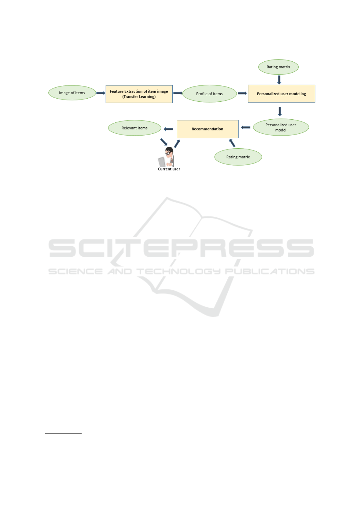
Figure 1: Proposed architecture.

the same model to extract features from a new image

dataset. Secondly, it takes more power computing to

learn huge models on large datasets. Thirdly, to take

a long time to learn the network.

Therefore, we use Transfer Learning method to

extract features describing images of items in our

dataset. We generally observe that the initial layers

capture the generic features while the deeper ones

become more speciﬁc in features extraction. It con-

sists in exploiting pre-trained models on large com-

plex data sets. There are many CNN architectures

such as VGG, ConvNet (Simonyan and Zisserman,

2014), ResNet (Targ et al., 2016), etc. In the proposed

transfer learning method, we used VGG-16 and VGG-

19 as basic models (Simonyan and Zisserman, 2014),

previously pre-trained for feature extraction task from

ImageNet dataset

. ImageNet is a dataset of over 15

million labeled high-resolution images belonging to

roughly 22,000 categories. Moreover, it is organized

according to the WordNet hierarchy. We use convo-

lutional layers of two models to extract features from

our dataset, and we eliminate fully connected layers

for classiﬁcation task. Therefore, VGG architecture

for the two pre-trained models is a composite of ﬁve

blocks of convolutional layers, some of which are fol-

lowed by Max-Pooling layers.

The image is passed through a stack of convolu-

tional layers, where the ﬁlters were used with a very

small receptive ﬁeld: 3 × 3. In one of the conﬁgura-

tions, it also utilizes 2 × 2 convolution ﬁlters, which

can be seen as a linear transformation of the input

channels. The convolution stride is ﬁxed to 1 pixel,

the spatial padding of convolutional layer input is

such that the spatial resolution is preserved after con-

http://www. image-net.org/

volution, i.e. the padding is 1-pixel for 3 × 3 convo-

lutional layers. Spatial pooling is carried out by ﬁve

max-pooling layers, which follow some of the con-

volutional layers. Max-pooling is performed over a

3 × 3 pixel window, with stride 2. In the VGG16: 13

convolutional layers. In the VGG19 model: 16 convo-

lutional layers. The width of convolutional layers (the

number of channels) is rather small, starting from 64

in the ﬁrst layer and then increasing by a factor of 2

after each max-pooling layer, until it reaches 512.

3.2.2 Dimension Reduction

The dimension reduction methods make it possible

to project the features into a reduced dimension in

order to deal with the scalability problems (Schafer

et al., 2007). Several techniques exist in the litera-

ture for reducing the dimension of a matrix. (Elkahky

et al., 2015) used Top-K features dimension reduction

technique, such as selecting the most relevant Top-K

features (eliminating non-signiﬁcant features with a

high zero rate). In addition, they use RBM

to reduce

the size to manage large-scale datasets. (Desrosiers

and Karypis, 2011) used other methods such as SVD

(Koren, 2008), that is to reduce the dimension of rat-

ing matrix, or to reduce the dimension of similarity

matrix. (Wang et al., 2016) used an Auto-Encoder

(AE) to reduce the size of dataset and compare this

technique with different dimension reduction tech-

niques.

The number K of features thus obtained may be

very high. It would be interesting to be able to re-

duce the K dimension of the MIP matrix by reducing

Restricted Boltzmann Machines

Singular Value Decomposition

WEBIST 2020 - 16th International Conference on Web Information Systems and Technologies

the number of features and thus deal with the scala-

bility problems. We choose to reduce the number of

features of the MIP (Matrix Items Proﬁle) using as

techniques the SVD and Top-K features.

We propose as a ﬁrst solution, to apply a Top-K

features, this technique selects the most relevant fea-

tures. More speciﬁcally, we eliminated features with

a number of zero greater than a given threshold NF

that is determined empirically.

Singular Value Decomposition (SVD) allows us

to project a dimension of the matrix (either rows l or

columns c) onto another dimension deﬁned by latent

variables described by the singular values of initial

matrix. The dimension of the projection is deﬁned

by the number of singular values of the initial matrix

which is equal to the minimum between l and c. La-

tent semantic analysis (LSA) reduces the projection

dimension by keeping only the largest R singular val-

ues.

We propose as a second solution, to apply a Latent

Semantic Analysis (LSA) (Dumais, 2004) of rank R

of MIP matrix. The rank R is well below the number

of features (R << |F|). LSA uses a truncated SVD

keeping only the R largest singular values and their

associated vectors. So, the rank-R approximation ma-

trix of the MIP matrix is provided by formula (2)

MIP ≈ I

J,R

∗ Σ

R,R

∗V

R,|F|

(2)

The rows in I

are the item vectors in LSA space

and the rows in V are the feature vectors in LSA

space. Thus, each item is represented in the LSA

space by a set of R latent variables instead of the fea-

tures of F.

3.3 Personalized User Modeling

In this section, we will present the second component

allowing personalized user modeling. The idea is to

build a new user proﬁle.

INPUT:

• Items proﬁle modeled by MIP result of ﬁrst com-

ponent.

• Usage data is represented by rating matrix Mv

having L rows and N columns. The lines repre-

sent the users and the columns represent the items.

Ratings are deﬁned on a scale of values. The rat-

ing matrix has missing value rate exceeding 95%,

where missing values are indicated by a ”?”, v

u,i

the rating of user u for item i, given by (Table 2)

OUTPUT: At the end of personalized user model-

ing, we obtain a personalized user model which is

Table 2: Rating Matrix (Mv).

1 . . . i . . . N

1 v

? v

. ?

. ? ?

u ? .. . v

.. . ?

. ? ?

L v

? v

represented by a matrix which we will call “Matrix

User Proﬁle ” (MU P

L,K

) without missing values, hav-

ing L rows representing the users and K columns

representing the features. This proﬁle deﬁnes user

preferences for the extracted features describing the

items based on their assessments for these same items.

MUP(u, f ): represents the utility of feature f for user

u as shown in (Figure 3).

Table 3: Personalized user model (Matrix of User Pro-

ﬁle(MUP)).

. . . f

1 f

1 j

u .. . f

u j

. . .

L f

L j

Personalized User Modeling. The idea is to infer the

utility of each feature of items (the result of compo-

nent 1) for each user. To do this we were inspired by

(Ben Ticha et al., 2013) which gives different formu-

las for calculating matrix of user proﬁles. We used

the formula which gave better results (see following

equation (3)).

MUP

(u, j)

∑

i∈I

relevant

u, j

× MIP

(i, j)

(3)

Computing I

relevant

We denote by I

relevant

the set of relevant items of user

u. To compute I

relevant

, we used the formula given in

(Ben Ticha, 2015). An item i is relevant for a user u

of U if it satisﬁes the following two conditions:



∈ [v

min

..v

max

] and v

neutral

max

relevant

= {i ∈ I

/ v

≥ v

and v

> v

neutral

}

(4)

Where v

indicates the average of rating. Using the

user’s average vote as a threshold to determine the rel-

evance of an item has two advantages. The ﬁrst is to

avoid adding a new parameter. The second is the per-

sonalization of the threshold which allows taking into

account the variation in the attribution of the marks

since all the users do not rate in the same way.

Transfer Learning to Extract Features for Personalized User Modeling

3.4 Recommendation

Among the existing collaborative approaches, CF al-

gorithms based on the K-Nearest-Neighbors algo-

rithm (Desrosiers and Karypis, 2011) are very pop-

ular because of their simplicity, their efﬁciency, and

their ability to produce relevant personalized recom-

mendations. The idea is to take advantage of the ef-

ﬁciency and simplicity of these algorithms to make

recommendations using the Personalized User Model

to determine the nearest neighbors of the current user.

The personalized user model is used to compute

similarities between users. Similarities are used to se-

lect the K nearest neighbors of the current user in a

user-based collaborative ﬁltering algorithm (Resnick

et al., 1994).

The User Proﬁle u (PU

) is represented by index

line u in User Proﬁle matrix (MUP) modeling the per-

sonalized model of users. Computing the similarity

between two users then amounts to calculating the

correlation between their two proﬁles. In our case, the

user proﬁle u (PU

) models the importance of the hid-

den features for the user u. The Cosine is utilized for

calculating the correlation between two users u and v.

It is deﬁned by the formula (5).

sim(u,v) = cos(

) =

|| ||

(5)

To compute predictions of rate value of an item i not

observed by the current user u

, we applied the for-

mula (6) keeping only the K nearest neighbors. The

similarity between u and u

being determined in our

case from their user proﬁles applying the formula (5).

pred(u

,i) = ¯v

∑

k nearest neighbors

sim(u

,u)(u

− ¯v

)

∑

k nearest neighbors

|sim(u

,u)|

(6)

The rating prediction in our approach is calculated by

applying user-based collaborative ﬁltering algorithm.

In the standard algorithm, the similarity between

users is calculated from rating matrix. In our case,

we use MUP matrix modeling the personalized users

proﬁle to calculate the similarity between users.

Our approach provides solutions to the scalability

problem. The ﬁrst two components, namely feature

extraction and personalized user modeling, are exe-

cuted in ofﬂine mode. To reduce the time complexity

of computing the rating prediction, the determination

of K nearest neighbors of each user is also computed

in ofﬂine mode, keeping only the k nearest to them.

The calculation of predictions for the current user is

executed in real-time during his interaction with e-

service (Figure2).

4 PERFORMANCE STUDY

A recommendation algorithm aims to improve the

usefulness of an e-service towards its users by in-

creasing their satisfaction. Thus, measuring user sat-

isfaction in terms of recommendation represents an

important evaluation criterion for any recommenda-

tion algorithm.

To evaluate our approach, we opted for ofﬂine

evaluation mode. The ofﬂine evaluation allows the

performance of several recommendation algorithms

to be compared objectively. We have adopted an

empirical approach. The performances of our ap-

proach were analysed through different experiments

on datasets.

We evaluated the performance of our approach

by measuring the accuracy of the recommendations,

which measures the capacity of a recommendation

system to predict recommendations that are relevant

to its users. We measured the accuracy of the pre-

diction by calculating the Root Mean Square Error

(RMSE) (Herlocker et al., 2004), which is the most

widely used metric in CF research literature.

RMSE =

∑

(u,i)∈T

(pred(u, i) − v

)

|T |

(7)

Where T is the set of couples (u,i) of R

test

for which

the recommendation system predicted the value of the

vote. It computes the average of the square root dif-

ference between the predictions and true ratings in the

test data set, lowers the RMSE is, better the accuracy

of predictions.

4.1 Experimental Datasets

We experimented our approach to real data from

two data sets. For the item content data, we used

the TMDb

(The Movie Database) dataset to extract

movie posters. TMDb provides the content of items

data set and contains 10 590 moviet posters with an

image size of 500 by 750.

We used the HetRec 2011 dataset of the Movie-

Lens recommender system

(IMDB, 2019) that links

the movies of MovieLens dataset with their cor-

responding web pages at Internet Movie Database

(IMDb), which contain user ratings. The HetRec-

2011 dataset provides the usage data set and contains

1,000,209 explicit ratings of approximately 3,900

movies made by 6,040 users with approximately 95%

of missing values.

https://www.themoviedb.org/

https://grouplens.org/datasets/hetrec-2011/

WEBIST 2020 - 16th International Conference on Web Information Systems and Technologies

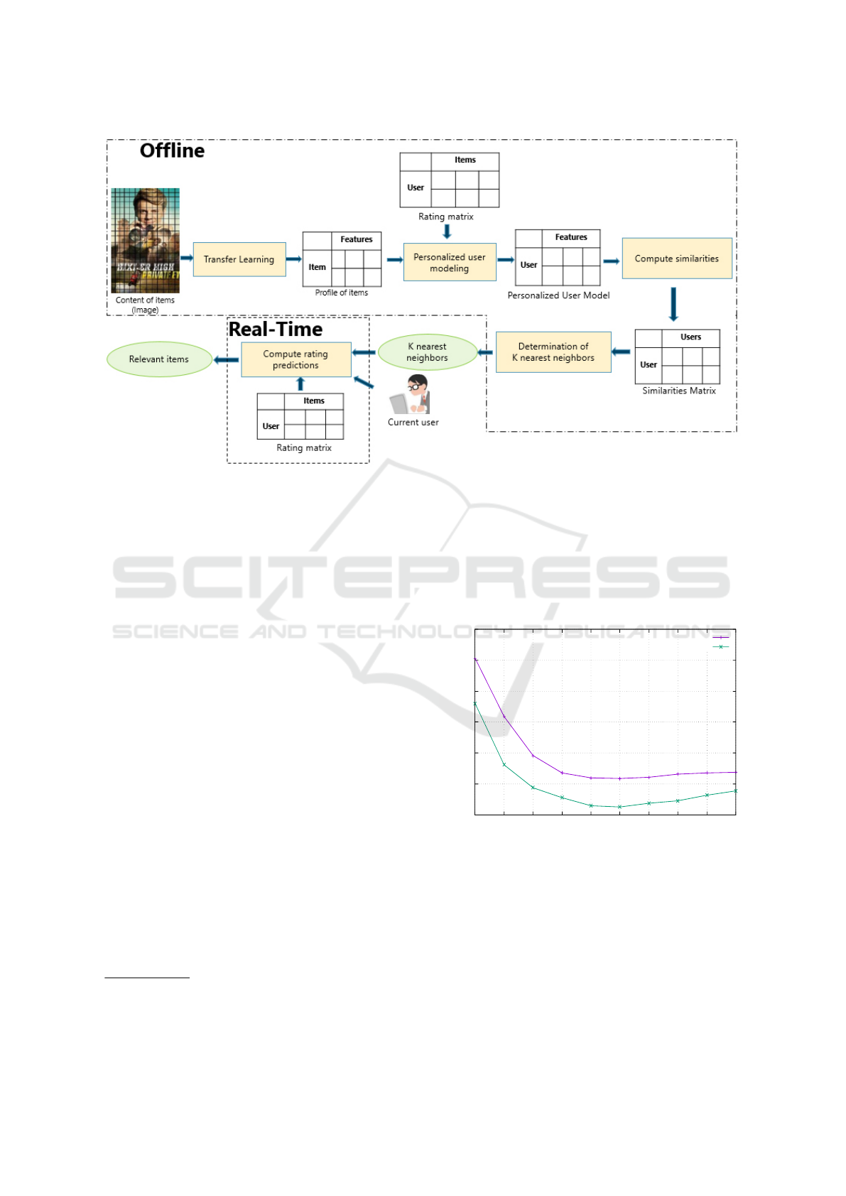
Figure 2: Synthesis of our approach.

The usage data set has been sorted by the times-

tamps, in ascending order, and has been divided into a

training set (including the ﬁrst 80% of all ratings) and

a test set (the last 20% of all ratings). Thus, ratings of

each user in the test set have been assigned after those

of the training set.

4.2 Performance Evaluation of Features

Extraction with VGG Models

To evaluate our approach, ﬁrstly, we started by fea-

tures extraction, and we took all the features extracted

of transfer learning. We used the pre-trained models

VGG16 and VGG19 for transfer learning technique

in the ﬁrst component 3.2 (features extraction from

movie posters) available included in the library keras

with Python programming language

with version

3.7 and run on TensorFlow

This technique gives us proﬁle item modeled by

Matrix Item Proﬁle (MIP) containing the latent fea-

tures for each movie poster i. Items in the row and

the features of each item in the column. Each element

has the importance of feature f for each item i which

is a value between [0.100].

The precisions of the two models (VGG16 and

VGG19) are shown in Figure 3. The RMSE is plot-

ted against the number K of neighbors. In all cases,

the RMSE converges between 50 and 60 neighbors.

https://keras.io/

https://www.python.org/

https://www.tensorﬂow.org/

The accuracy of predictions ratings of the VGG19

model is higher than that observed by VGG16, for

all the neighbors. The best performance is obtained

by VGG19 whose RMSE value is equal to 0.9263

for 60 neighbors. For VGG16, the best performance

is obtained for the same number of neighbors with a

RMSE equal to 0.9309.

0.925

0.93

0.935

0.94

0.945

0.95

0.955

10 20 30 40 50 60 70 80 90 100

RMSE

Number of nearest neighbors

VGG16

VGG19

Figure 3: Evaluation with VGG models.

4.3 Performance Evaluation of

Dimension Reduction

4.3.1 Dimension Reduction with Top-K Features

To improve the performance of our approach, we re-

duced the size of the MIP (Matrix Items Proﬁle) by

selecting the most relevant features. More speciﬁ-

Transfer Learning to Extract Features for Personalized User Modeling

cally, we eliminated the features with a number of

zero greater than a given threshold = ”NF

zero

” that is

determined empirically. Where threshold is the rate

% of zero in the features.

Figure 4 illustrates the performance of selecting

the features ”NF

zero

” in ﬁxing K = 60 of K-Nearest-

Neighbors. In fact, for the VGG16 model, the initial

number of features is equal to 25028, the selection of

features from the item proﬁle matrix (MIP) is 0%, the

accuracy of recommendations which has reached the

value of RMSE = 0.9309. On the other hand, the ac-

curacy of recommendations of VGG19 model reached

the value of RMSE = 0.9263 of the accuracy of rec-

ommendations.

Figure 5 illustrates the performances of dimension

reduction. The performances of VGG19 model are

compared with those obtained without reduction of

the dimension (plot in green). The reduction in size

degrades the performance of our approach. Table 4

gives the rate of dimension reduction corresponding

tothreshold = ”NF

zero

” and number of latent features

F of VGG19 model.

0.916

0.918

0.92

0.922

0.924

0.926

0.928

0.93

0.932

0.934

0 10 20 30 40 50 60 70 80

RMSE

Threshold (%)

With K=60

VGG19

VGG16

Figure 4: Performance evaluation of selecting the relevant

Top-K features.

The feature selection of the matrix item proﬁle in-

creases the accuracy until its rank reaches a thresh-

old value of the Percentage selection of features from

which the accuracy begins to decrease. This obser-

vation remains the same for the other VGG19 model.

The threshold value for the accuracy of recommenda-

tions of the VGG16 model is equal to RMSE = 0.9217

corresponds to 40% of the selection of features from

the Matrix Item Proﬁle (MIP). On the other hand, in

the VGG19 model, the threshold value for the accu-

racy of recommendations is equal to RMSE = 0.9165

corresponds to 50% of the selection of features.

The dimension reduction made possible not only

to reduce the size of the model and thus to improve

its performance in terms of scalability, but also to im-

prove its performance in terms of precision of the rec-

ommendations.

4.3.2 Dimension Reduction with LSA

In Figure 6, the RMSE has been plotted with respect

to the LSA rank. We reduce the size of MSI in ﬁxing

k = 60 of K-Nearest-Neighbors of the VGG-19 model

by applying a LSA with rank R. The performances

are compared with those obtained without reduction

of the dimension (curve in green).

The factorization of a matrix MPI (10 590, 25028)

is the application an SVD, so the number of latent

features is equal to R = min (10 590, 25028). The

factorization of MPI matrix resulted in a degradation

of precision of the recommendations which reached

the value of RMSE = 0.9477 for R = 10 590 against

RMSE = 0.9263 without factorization. The dimen-

sion reduction increases the precision until reaching

a threshold value of R from which the precision be-

gins to decrease. The optimum is reached for R equal

to 1000 with an RMSE = 0.9239 slightly better than

that obtained without dimension reduction (RMSE =

0.9263). Although the LSA doesn’t improve the ac-

curacy, dimension reduction is signiﬁcant. Thus, it al-

lows to reduce the cost of users similarity computing,

specially when the number of features is very high.

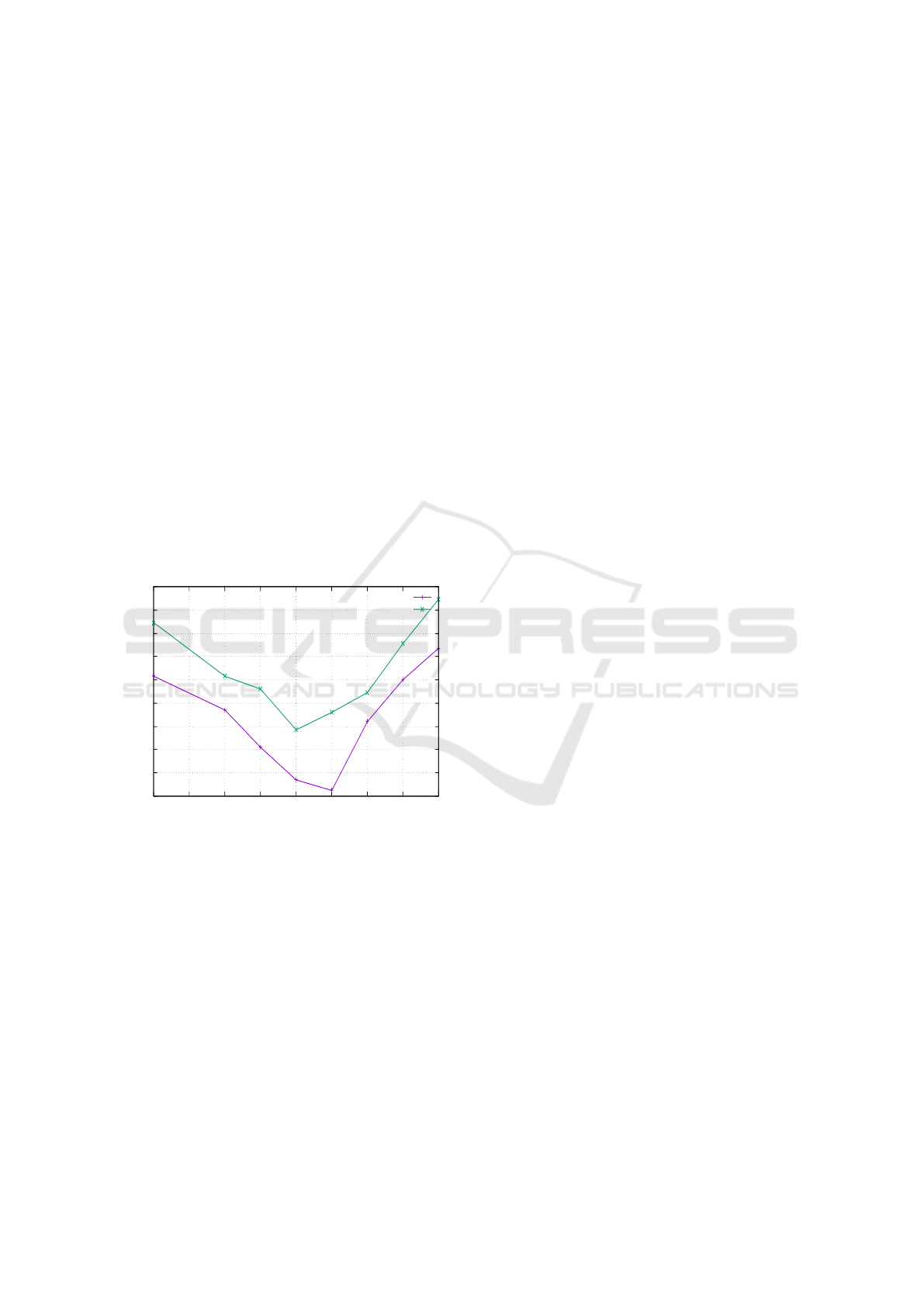
4.4 Comparative Results of Our

Approach against Other

Approaches based on CF

In Figure 7, the RMSE has been plotted with

respect to the number K of neighbors in the k-

Nearest-Neighbor algorithm, with K ∈ [10, 100].

We compared the performance of our approach

using VGG19 model compared to a “User Semantic

Collaborative Filtering” approach (Ben Ticha, 2015)

which treated with different text attributes describing

movies (Genre, Origin).

We represented the performances of four exper-

iments on the same data set: the Genre of movie

attribute (e.g., comedy, drama) represented by the

“Genre” plot, the Origin of movie attribute (the coun-

try of movie origin) represented by the “Origin” plot,

the movie poster with dimension reduction with Top-

K features in size represented by the “VGG19 with re-

duction” plot and the movie poster without reduction

of the dimension represented by the “VGG19 without

reduction” plot.

WEBIST 2020 - 16th International Conference on Web Information Systems and Technologies

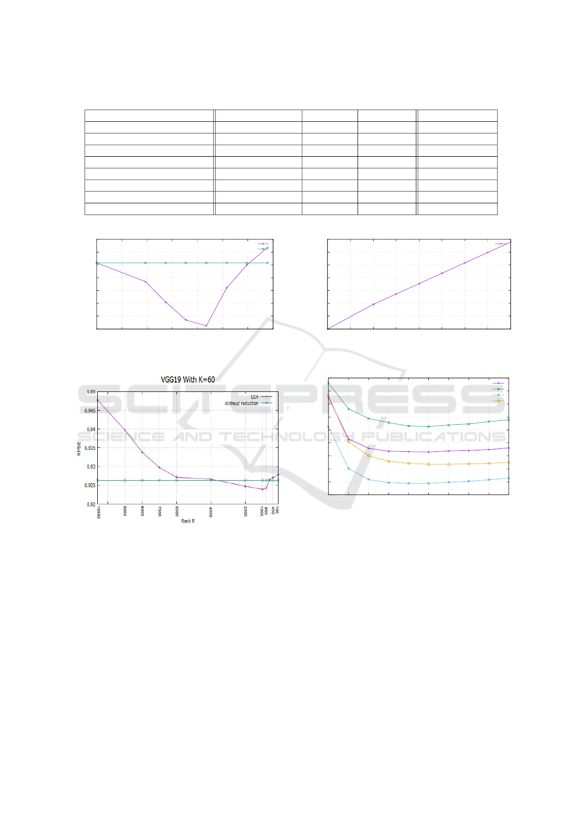
Table 4: Dimension reduction with Top-K features of VGG19 model.

% Threshold : ”NF

zero

” % Reduction F RMSE Gain RMSE

0% 0% 25028 0.9263 ±0.0000

20% 19.27% 20204 0.9234 +0,0029

30% 27.35% 18183 0.9202 +0.00161

40% 35.42% 16163 0.9174 +0,0089

50% 43.5% 14142 0.9165 +0,0098

60% 51.57% 12122 0.9224 +0,0039

70% 59.64% 10102 0.9260 +0,0003

80% 67.77% 8081 0.9287 −0,0024

0.916

0.918

0.92

0.922

0.924

0.926

0.928

0.93

0 10 20 30 40 50 60 70

RMSE

Dimension Reduction (%)

VGG19 With K=60

With reduction

Without reduction

0 10 20 30 40 50 60 70 80

Dimension Reduction (%)

Threshold (%)

VGG19 With K=60

VGG19

Figure 5: Performance evaluation of dimension reduction with Top-K features.

10590

9000

7000

8000

6000

800

400

4000

2000

1000

100

90009000

800

1000

800

1000

400400

70007000

Figure 6: Performance evaluation of LSA.

By analyzing the plots of the graph, we see that

all the plots have the same appearance, the RMSE de-

creases to a given value of K (The Nearest Neighbors)

then increase. All the plots converge for N between

50 and 60 neighbors. The accuracy of the genre rat-

ing predictions is higher than that observed by Ori-

gin, which themselves are higher to those recorded by

our approach which processes the image content of

items using VGG19 and this for all neighbors. The

best performance is obtained by the movie Genre at-

tribute whose RMSE value is equal to 0.9035 for 60

neighbors, again of the order of 2 points compared to

our approach whose RMSE is equal to 0.9263 for the

same number of neighbors.

0.9

0.905

0.91

0.915

0.92

0.925

0.93

0.935

0.94

0.945

10 20 30 40 50 60 70 80 90 100

RMSE

Number of nearest neighbors

VGG19 With reduction

VGG19 Without reduction

Gender

Origin

Figure 7: Comparative results of our approach against other

approaches based CF.

In conclusion, we can say that the best perfor-

mance which deals with the textual data describing

the item (Genrer, Origin). The results of our approach

are acceptable compared to the results of (Ben Ticha,

2015) which explains this by the fact that the poster

of a movie has an importance in the preferences of the

users and it may not be discriminating enough as the

genre or origin. Thus, we used transfer learning with

the pre-trained VGG-16 and VGG19 models with Im-

ageNet dataset but if we will build a model Convo-

lutional Neural Network (CNN) of classiﬁcation task

by trained from the movie poster dataset, then we will

apply transfer learning of our dataset. Perhaps in the

case, the results can be better.

Transfer Learning to Extract Features for Personalized User Modeling

5 CONCLUSION AND FUTURE

WORK

In this paper, we have proposed to apply transfer

learning to extract latent features of images describing

items. We have used the resulting model for person-

alized user modeling by inferring user preferences for

latent features of images from the history of their pref-

erences for items and thus building the user model.

The personalized model obtained was then user used

collaborative ﬁltering algorithm on users to make rec-

ommendations.

We evaluated the performance of our approach

by applying two different feature extraction models

VGG16, VGG19. To improve the performance of

our approach, we applied two method Top-K features

and LSA for the reduction dimension. Finally, we

compared the accuracy of our approach to other ap-

proaches based on hybrid ﬁltering which deals with

different text attributes describing items.

As a fertile interdisciplinary research area of rec-

ommendation and transfer learning, there are various

exciting directions worth further exploration in our

approach. In future work, we will include several ma-

jor directions extension of the application domain and

apply other dimension reduction algorithms.

We have experimented with our approach in the

area of movie recommendation and more speciﬁcally

MovieLens datasets. However, the performance of a

recommendation algorithm may vary depending on

the data used or the application domain (Shani and

Gunawardana, 2011). It is for this reason that it would

be interesting to conﬁrm our conclusions by experi-

menting with our approach to other ﬁelds of applica-

tions such as the recommendation of ready meals or

clothing for example.

To reduce the size of the model representing the

items features, at the end of the transfer learning for

features extraction, we opted for the ﬁltering of the

features by eliminating the least relevant, having a

rate of zero greater than a given threshold ( Top-K

features) and LSA for dimension reduction. Besides,

there are several methods of dimension reduction al-

lowing to project the features in a reduced dimension.

It is also interesting to use deep learning techniques

such as the Restricted Boltzmann Machines (RBM)

or the AutoEncoder (AE).

REFERENCES

Adomavicius, G. and Tuzhilin, A. (2005). Toward the next

generation of recommender systems: A survey of the

state-of-the-art and possible extensions. IEEE Trans-

actions on Knowledge & Data Engineering, (6):734–

749.

Ben Ticha, S. (2015). Recommandation Personnalis

ee Hy-

bride. PhD thesis, Facult

e des Sciences de Tunis.

Ben Ticha, S., Roussanaly, A., Boyer, A., and Bsa

ıes, K.

(2013). Feature frequency inverse user frequency

for dependant attribute to enhance recommendations.

In The Third Int. Conf. on Social Eco-Informatics -

SOTICS, Lisbon, Portugal. IARIA.

Bengio, Y. et al. (2009). Learning deep architectures for

ai. Foundations and trends

 in Machine Learning,

2(1):1–127.

Biadsy, N., Rokach, L., and Shmilovici, A. (2013). Trans-

fer learning for content-based recommender systems

using tree matching. In International Conference on

Availability, Reliability, and Security, pages 387–399.

Springer.

Chu, W.-T. and Tsai, Y.-L. (2017). A hybrid recom-

mendation system considering visual information for

predicting favorite restaurants. World Wide Web,

20(6):1313–1331.

Cui, Q., Wu, S., Liu, Q., Zhong, W., and Wang, L. (2018).

Mv-rnn: A multi-view recurrent neural network for

sequential recommendation. IEEE Transactions on

Knowledge and Data Engineering.

de Souza, G. B., da Silva Santos, D. F., Pires, R. G., Marana,

A. N., and Papa, J. P. (2019). Deep features extrac-

tion for robust ﬁngerprint spooﬁng attack detection.

Journal of Artiﬁcial Intelligence and Soft Computing

Research, 9(1):41–49.

Deng, L., Yu, D., et al. (2014). Deep learning: methods

and applications. Foundations and Trends

 in Signal

Processing, 7(3–4):197–387.

Desrosiers, C. and Karypis, G. (2011). A comprehensive

survey of neighborhood-based recommendation meth-

ods. In Recommender systems handbook, pages 107–

144. Springer.

Dumais, S. T. (2004). Latent semantic analysis. An-

nual review of information science and technology,

38(1):188–230.

Elkahky, A. M., Song, Y., and He, X. (2015). A multi-

view deep learning approach for cross domain user

modeling in recommendation systems. In Proceed-

ings of the 24th International Conference on World

Wide Web, pages 278–288. International World Wide

Web Conferences Steering Committee.

Herlocker, J. L., Konstan, J. A., Terveen, L. G., and Riedl,

J. T. (2004). Evaluating collaborative ﬁltering recom-

mender systems. ACM Transactions on Information

Systems (TOIS), 22(1):5–53.

Hinton, G. E. and Salakhutdinov, R. R. (2006). Reducing

the dimensionality of data with neural networks. sci-

ence, 313(5786):504–507.

IMDB (2019). https://www.imdb.com/, consulted juin

2019.

Karatzoglou, A. and Hidasi, B. (2017). Deep learning

for recommender systems. In Proceedings of the

eleventh ACM conference on recommender systems,

pages 396–397. ACM.

WEBIST 2020 - 16th International Conference on Web Information Systems and Technologies

Karpathy, A. et al. (2016). Cs231n convolutional neural

networks for visual recognition. Neural networks, 1.

Koren, Y. (2008). Factorization meets the neighborhood:

a multifaceted collaborative ﬁltering model. In Pro-

ceedings of the 14th ACM SIGKDD international con-

ference on Knowledge discovery and data mining,

pages 426–434. ACM.

Lei, C., Liu, D., Li, W., Zha, Z.-J., and Li, H. (2016). Com-

parative deep learning of hybrid representations for

image recommendations. In Proceedings of the IEEE

Conference on Computer Vision and Pattern Recogni-

tion, pages 2545–2553.

Nguyen, H. T., Wistuba, M., and Schmidt-Thieme, L.

(2017). Personalized tag recommendation for images

using deep transfer learning. In Joint European Con-

ference on Machine Learning and Knowledge Discov-

ery in Databases, pages 705–720. Springer.

Rashid, M., Khan, M. A., Sharif, M., Raza, M., Sarfraz,

M. M., and Afza, F. (2019). Object detection and clas-

siﬁcation: a joint selection and fusion strategy of deep

convolutional neural network and sift point features.

Multimedia Tools and Applications, 78(12):15751–

15777.

Resnick, P., Iacovou, N., Suchak, M., Bergstrom, P., and

Riedl, J. (1994). Grouplens: an open architecture for

collaborative ﬁltering of netnews. In Proceedings of

the 1994 ACM conference on Computer supported co-

operative work, pages 175–186.

Schafer, J. B., Frankowski, D., Herlocker, J., and Sen, S.

(2007). Collaborative ﬁltering recommender systems.

In The adaptive web, pages 291–324. Springer.

Shani, G. and Gunawardana, A. (2011). Evaluating recom-

mendation systems. In Recommender systems hand-

book, pages 257–297. Springer.

Sharif, M., Attique Khan, M., Rashid, M., Yasmin, M.,

Afza, F., and Tanik, U. J. (2019). Deep cnn and ge-

ometric features-based gastrointestinal tract diseases

detection and classiﬁcation from wireless capsule en-

doscopy images. Journal of Experimental & Theoret-

ical Artiﬁcial Intelligence, pages 1–23.

Simonyan, K. and Zisserman, A. (2014). Very deep con-

volutional networks for large-scale image recognition.

arXiv preprint arXiv:1409.1556.

Targ, S., Almeida, D., and Lyman, K. (2016). Resnet

in resnet: Generalizing residual architectures. arXiv

preprint arXiv:1603.08029.

TMDB (2019). The movie database, https://www.

themoviedb.org/, consulted juin 2019.

Wang, Y., Yao, H., and Zhao, S. (2016). Auto-encoder

based dimensionality reduction. Neurocomputing,

184:232–242.

Wei, Y., Xia, W., Huang, J., Ni, B., Dong, J., Zhao, Y., and

Yan, S. (2014). Cnn: Single-label to multi-label. arXiv

preprint arXiv:1406.5726.

Yu, W., Zhang, H., He, X., Chen, X., Xiong, L., and Qin,

Z. (2018). Aesthetic-based clothing recommendation.

In Proceedings of the 2018 World Wide Web Confer-

ence, pages 649–658. International World Wide Web

Conferences Steering Committee.

Zhang, S., Yao, L., Sun, A., and Tay, Y. (2019). Deep

learning based recommender system: A survey and

new perspectives. ACM Computing Surveys (CSUR),

52(1):5.

Zhou, J., Albatal, R., and Gurrin, C. (2016). Applying vi-

sual user interest proﬁles for recommendation and per-

sonalisation. In International Conference on Multime-

dia Modeling, pages 361–366. Springer.

Transfer Learning to Extract Features for Personalized User Modeling