
Validating Results of 3D Finite Element Simulation for Mechanical
Stress Evaluation using Machine Learning Techniques
Alexander Smirnov
1a
, Nikolay Shilov
2b
, Andrew Ponomarev
1c
,
Thilo Streichert
3
, Silvia Gramling
3d
and Thomas Streich
3e
1
SPIIRAS, 14
th
Line, 39, St. Petersburg, Russia
2
ITMO University, Kronverksky pr., 49, St. Petersburg, Russia
3
Festo SE & Co. KG, Ruiter Str., 82, Esslingen, Germany
Keywords: Artificial Intelligence, 3D Simulation Data, Mechanical Stress Evaluation, Geometric Features, Resnet18,
VoxNet.
Abstract: When a new mechanical part is designed its configuration has to be tested for durability in different usage
conditions (‘stress evaluation’). Before real test samples are produced, the model is checked analytically via
3D Finite Element Simulation. Even though the simulation produces good results, in certain conditions these
could be unreliable. As a result, validation of simulation results is currently a task for experts. However, this
task is time-consuming and significantly depends on experts’ competence. To reduce the manual checking
effort and avoid possible mistakes, machine learning methods are proposed to perform automatic pre-sorting.
The paper compares several approaches to solve the problem: (i) machine learning approach, relying on
geometric feature engineering, (ii) 2D convolutional neural networks, and (iii) 3D convolutional neural
networks. The results show that usage of neural networks can successfully classify the samples of the given
training set.
1 INTRODUCTION
When a new mechanical part is designed, it has to be
tested for durability in different usage conditions
(‘stress evaluation’). In order to save on time and
expenses, the model is usually checked analytically
before real test samples are produced. However,
automated simulations sometimes deliver results that
require expert knowledge for interpretation.
Currently, experts validate if the results are reliable
and detect the nonreliable ones (fig. 1, a). This is a
time-consuming and prone to errors process.
In case of finite element simulations (Reddy,
2009), nonreliable results (“failures”) can arise from,
for example:
Overlapping components in the imported CAD
file,
Contact of different (rigid) components or
a
https://orcid.org/0000-0001-8364-073X
b
https://orcid.org/0000-0002-9264-9127
c
https://orcid.org/0000-0002-9380-5064
d
https://orcid.org/0000-0002-8197-3538
e
https://orcid.org/0000-0002-0191-6366
Equal treatment of tensile and compressive stress.
In order to reduce the manual checking efforts and
also to avoid checking mistakes, training of machine
learning models that allow automatic pre-sorting is
proposed within the scope of this research study (fig.
1, b).
The challenge of this classification task is that the
simulation results are given as unstructured 3D point
clouds, so common frameworks for processing
regular data, e.g. for image recognition, cannot be
applied directly. That is why different problem
specific approaches have to be studied.
The research question considered in the paper is if
the classification of reliability (automated validation)
of the 3D finite element simulation results can be
done using AI and which AI approaches can provide
for acceptable results.
The paper compares three approaches to solve the
Smirnov, A., Shilov, N., Ponomarev, A., Streichert, T., Gramling, S. and Streich, T.
Validating Results of 3D Finite Element Simulation for Mechanical Stress Evaluation using Machine Learning Techniques.
DOI: 10.5220/0010108500130023
In Proceedings of the International Conference on Innovative Intelligent Industrial Production and Logistics (IN4PL 2020), pages 13-23
ISBN: 978-989-758-476-3
Copyright
c
2020 by SCITEPRESS – Science and Technology Publications, Lda. All rights reserved
13
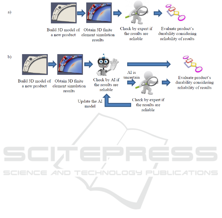
Figure 1: The process of evaluating new product’s durability: current (a), desired (b).
problem using different machine learning techniques:
1) machine learning approach, relying on geometrical
feature engineering, 2) 2D convolutional neural
networks, and 3) 3D convolutional neural networks.
The paper is strucutred as follows. The next
section defines the problem at hand. It is followed by
the state of the art review. Sections 4-6 repesent the
AI training and classification results for the above
mentioned techniques. The results are compared and
discussed in section 7. The conclusions summarize
the findings and outline the future research directions.
2 PROBLEM DEFINITION
The source data for the classification problem is
stored in VTU mesh files (Kitware Inc., 2005) with
different number of points per inch depending on the
curvature of a particular fragment of the model (less
points on smooth surfaces and more points for
curves). An average number of vertices in a model is
around 5000 but it differs significantly from model to
model. Due to symmetry, models are given as 1/4 part
or 1/2 part of a component. If the components had no
symmetry properties, the model would have
represented the whole part.
The locations of the vertices of a sample are set
before the simulation is conducted. The output of the
simulation are so-called safety factor values for each
vertex. This safety factor (SF) value is defined as the
relationship between an allowable mechanical load
and a given mechanical load. That means, the higher
the SF, the more stable the simulated component is.
That is why the SF is used as a metric to decide if a
component fulfils the mechanical requirements of the
development process. Therefore, the minimal SF
value has to lie above a certain threshold. Validation of
the reliability of this minimal SF is the problem at
hand. In order to automate it, within the scope of this
research work machine learning models have been
developed to validate if this minimum is reliable or not.
The reliability check is then applied iteratively: If the
global minimum is not reliable, the second lowest local
minimum is validated and so on until a reliable
minimum is found. This SF minimum has to lie above
the threshold to be mechanically stable. Otherwise, the
construction needs to be re-engineered.
In the dataset of this research study, the label
refers to the global minimum, so only the global
minimum is classified. Since the global minimum is
the easiest to find and the patterns for classification
are the same for other local minima, this study is
focused on the classification of the global minimum.
The the test set consisting of 814 simulation
results was manually classified by an expert based on
the evaluation of the reliability of the global
minimum so that 304 samples were considered as
reliable (“reliable samples”), and 510 samples as
nonreliable (“nonreliable samples”). The nonreliable
samples are split into 3 types of failures (failure
modes): 142, 115, and 253 samples respectively.
However, in the presented research only two labels are
IN4PL 2020 - International Conference on Innovative Intelligent Industrial Production and Logistics
14

used: reliable and unreliable. Classification of samples
into failure modes is still the subject of future research.
3 STATE-OF-THE-ART REVIEW
The considered task is rather unique, and no “of the
box” solutions or methods have been found. As a
result, the paper presents approaches for classifying
models of 3D objects. One can read on advances in
3D object classification in (Ahmed et al., 2018;
Ioannidou et al., 2017). Based on these, all
approaches to 3D object classification can be split
into the following groups:
Architectures exploiting descriptors extracted
from 3D data,
Architectures exploiting RGB data,
Architectures exploiting 3D data directly.
The first group of approaches is not directly
related to 3D object classification but follows the
generic approach of feature selection and application
of various models to the features and their
combinations (L. Ma et al., 2018; Wahl et al., 2003).
These models are less computationally expensive and
are preferable for tasks where they can be applied
successfully. However, they often cannot work well
for distinguishing between some complex shapes.
The second group of approaches is based on
application of various techniques to generating 2D
images out of 3D objects and their further
classification. These approaches can also be split into
two groups: (i) analysing various views, projections,
and cuts, and (ii) analysing images with depth
information. The advantage of these approaches is the
possibility to use well-studied 2D classification
techniques without the need to develop a new 3D
model. However, extensive application of such
techniques caused appearance of specialized multi-
view models (Su et al., 2015; Yavartanoo et al., 2019;
Zhou et al., 2020). The cut-based approaches are most
often used in medical domain since many medical
data, for example, tomography results, were
originally represented as cuts (Deng et al., 2018; Lu
et al., 2018; Z. Ma et al., 2018), however they are
applied in other domains as well (Qiao et al., 2018).
Analysing images with depth information (often
referred as RGB-D) is a very popular group of
approaches. They also had the advantage of applying
state-of-the-art 2D classification techniques to
classifying 3D objects but developed into a separate
group classification models (Feng et al., 2016;
Schwarz et al., 2015).
Direct analysis of 3D data can also be approached
from different perspectives. Classification of meshes
(Hanocka et al., 2019) and irregular point clouds
(Charles et al., 2017; Y. Wang et al., 2019) are
characterized by speed and absence of the need of
computation-intensive pre-processing since usually
engineering and design data (e.g., CAD models) are
stored in this form. Approaches based on analysis of
regular point clouds (voxel-based models) provide
better results “out-of-the-box”, for the price of
additional data pre-processing (Maturana & Scherer,
2015).
In the presented research one approach from each
group was tested: classification based on geometrical
feature engineering, 2D convolutional neural network
(Resnet18) for depth images, and 3D convolutional
neural network VoxNet. A number of models for
irregular point clouds have also been tested, but so far
their result were much worse than those presented so
they are not considered in the paper.
4 CLASSIFICATION BASED ON
GEOMETRIC FEATURES
4.1 Approach Description
The first approach is to build a classification model
that relies on geometrical feature engineering. As the
definition of the error modes is connected to some
geometric properties of the SF minimum point and its
neighbourhood, a set of features was proposed
describing the geometry of the neighbourhood of the
SF minimum. In particular, the features describe the
complexity of the SF minimum neighbourhood,
including two interpretations of mesh complexity:
1. Structural complexity, related to the number of
nodes and faces in the mesh.
2. Geometric complexity, describing how similar the
surface is to a “simple” shape (e.g., plane).
Structural complexity is quite easy to formalize
and evaluate. We created two groups of features:
cells_no_X (number of mesh cells in the SF minimum
neighbourhood of the given radius in millimetres) and
points_no_X (number of mesh nodes in the SF
minimum neighbourhood of the given radius in
millimetres). The corresponding features are
calculated by intersecting the input mesh with a
sphere of the particular radius positioned to the SF
minimum point and finding the properties of the
resulting mesh.
It is not clear in advance what is the size of the SF
neighbourhood that is the most informative to the
reliability classification. In order to understand that,
Validating Results of 3D Finite Element Simulation for Mechanical Stress Evaluation using Machine Learning Techniques
15

each feature was generated w.r.t. different sizes of
neighbourhood (sphere radiuses). For example, we
created the features “number of nodes in 1 mm radius
neighbourhood” (points_no_1), as well as in 2 mm
(points_no_2), 3 mm (points_no_3) radius
neighbourhoods and so on. It applies to all the
features (representing both structural and geometric
complexity).
The notion of geometric complexity is not so
straightforward to formalize. Therefore, several
features were introduced.
The first is the volume of the minimal oriented
bounding box of the neighbourhood of the specified
size (obb_volume_X). The intuition behind this
feature is that flat or slightly bent surfaces have a
bounding box with zero or close to zero volume,
while for curved surfaces the bounding box will be
(almost) close to a cube having relatively large
volume. Minimal oriented bounding boxes are
estimated with a help of trimesh library (Dawson-
Haggerty et al., n.d.).
The second group of features is generalized
variance of face normals (in the neighbourhood of the
specified size – gen_var_X), estimated according to
the following formula:
1
||
|
|
,
where – a set of vectors normal to mesh faces (each
vector is 3-dimensional), and
– is the mean normal.
The next group of features is the neighbourhood
convexity, estimated using the tangent plane,
containing the minimum SF point. In particular, there
are two groups of features, calculated using this tangent
plane. Features convexity1_X are defined as the mean
value of the plane equation for the neighbourhood
points, while convexity2_X features are defined as the
logarithm of the ratio of the number of points in the
positive subspace w.r.t. the tangent plane, to the
number of points in the negative subspace.
The features of the next group are rooted in the
notion of surface curvature. Specifically, we use the
notion of discrete gaussian curvature measure as
defined in (Cohen-Steiner & Morvan, 2003) and
implemented in trimesh library. This gives two
groups of features gauss_curv_X (the sum of the
discrete gaussian curvature of the nodes in the
specified neighbourhood) and gauss_curv_avgd_X
(mean discrete gaussian curvature of the specified
neighbourhood).
All the described groups of features characterize
the SF minimum neighbourhood of the given size in
millimetres. The last group of features describe the
closest possible neighbourhood of the SF minimum
node, given by the mesh structure – nodes reachable
from the SF minimum by one and two ‘hops’. This
gives features edgeness_min_1nbr,
edgeness_max_1nbr, edgeness_min_2nbr, and
edgeness_max_2nbr. In the name of these features
min and max correspond to minimal and maximal
values of the cosine of the angle between the normal
of faces situated in the given neighbourhood, and
1nbr and 2nbr suffixes correspond to the
neighbourhoods reachable in one and two hops from
the minimum SF point respectively. The complete list
of features is provided in the table 1.
4.2 Feature Importance Analysis
Feature importance analysis shows how informative
each feature is in the process of classification. In this
problem, the role of feature importance analysis is at
least twofold:
1. The features are very similar, they all try to
capture convexity in some sense. Which one is
better?
2. What neighbourhood size is the most
informative? This knowledge can help to keep the
model small and thus to speed up the processing.
Besides, understanding the size of the informative
neighbourhood may help to select
neighbourhoods used to train other ML methods.
Table 1: The list of features.
Feature Neighbourhood sizes, mm
cells_no_X 10, 8, 6, 5, 4, 3, 2, 1
points_no_X 10, 8, 6, 5, 4, 3, 2, 1
obb_volume_X 10, 8, 6, 5, 4, 3, 2, 1
gen_var_X 10, 8, 6, 5, 4, 3, 2, 1
convexity1_X 5, 4, 3, 2, 1
convexity2_X 5, 4, 3, 2, 1
gauss_curv_X 5, 4, 3, 2, 1
gauss_curv_avgd_X 5, 4, 3, 2, 1
edgeness_min_1nbr -
edgeness_max_1nbr -
edgeness_min_2nbr -
edgeness_max_2nbr -
To estimate feature importance we used null
importance method (Altmann et al., 2010; Grellier,
2018) in conjunction with feature importance
estimation procedures typical for the tree-based
learning algorithms.
The idea is as follows. The machine learning
algorithm leveraged for reliability classification is a
decision tree-based gradient boosting implemented in
CatBoost library (Yandex, 2020b). Decision tree-
based learning algorithms have an internal ability to
IN4PL 2020 - International Conference on Innovative Intelligent Industrial Production and Logistics
16

estimate feature importance, i.e. the impurity measure
(information or Gini) gain, which is obtained by the
splits that use the particular feature (Y. Y. Wang &
Li, 2008). Gradient boosting on decision trees
implemented in CatBoost is not an exception, as it
also estimates the importance of the input features by
how on average the prediction changes if the feature
value changes (Yandex, 2020a). However, feature
importance estimation is not always indicative of the
actual importance of the feature, especially in
multidimensional spaces and in the presence of noise.
The main problem is that it is usually is not clear what
level of impurity gain corresponds to some real
patterns in the data, and what gain can be learned even
from the noise.
The null importance method provides some kind
of a ‘reference point’ in assessing the importance. The
rationale behind the method is following. Let’s
consider a slightly modified learning dataset, where
feature f is replaced with its random permutation f*.
A learning algorithm can be applied to the modified
dataset and an importance of f* can be estimated in a
usual way. Further, as we repeat this process several
times, for each feature we can build an importance
distribution (null importance distribution). That
distribution essentially provides the required
‘reference point’ – if sampling the importance of the
feature f in its original ordering is likely to be sampled
from this distribution then the feature is actually no
more important than the random noise. On the other
hand, if the importance of the feature in its original
ordering is greater than the importance of most of the
permutations of this feature, it actually carries some
information about the target. This also gives a way to
measure the importance, e.g., by considering the ratio
of the importance of the original feature ordering to
the 3rd quartile of the null importance distribution.
Table 2 shows top 10 features estimated by the
described procedure. It can be seen from the table that
Table 2: Top 10 features according to the null importance
method.
Feature Importance
convexity1_4 5.5
convexity1_3 4.6
convexity1_5 4.0
convexity2_4 3.8
convexity2_3 3.8
convexity2_5 2.2
obb_volume_2 1.8
gauss_curv_avgd_2 1.3
convexity2_2 0.97
convexity2_1 0.95
only 5 features have importance greater than the 3
rd
quartile of the null importance distribution. The most
important features are various convexity indicators
applied to the SF minimum neighbourhoods of the
radius 3 mm and 4 mm. Smaller and larger
neighbourhoods are not so important.
5 CNN-BASED CLASSIFICATION
OF DEPTH IMAGES
The second approach is based on the representation
of the 3D models as 2D depth images and further
classification by a convolutional neural network. In
certain sense this representation can be considered as
surface model, where coordinates of an image point
correspond to the coordinates of the surface point
along two axes, and the depth colour can be
considered as the coordinate along the third axis.
Generation of the depth images has been done via
the following procedure. First, the fragment of a
given diameter around the analysed point (the point
with the minimal SF, fig. 2, a and b). Experiments
were carried out with radiuses of 2, 3, and 4 mm,
however for simplicity 3 mm radius is considered in
the descriptions below.
Then, the fragment is rotated so that the normal of
the analysed point would be oriented along axis Z
(pointing to the viewer in fig. 2, c).
In the presented example, one can see that in some
complex shapes, there can be fragments obstructing
the analysed point, and, as a result, it is not possible
to see the shape around it. For this purpose, a
procedure has been developed for removing such
obstructing fragments. It consists of two steps:
(1) remove all points whose normals are oriented to
opposite direction (cosine between the normals of
analysed point and checked point is negative);
(2) remove all fragments that are not connected to the
fragment containing the analysed point. The resulting
fragment is shown in fig. 2, d.
Finally, the depth map is built via measuring
distances between the fragment and nodes of a
224x224 grid located on a flat surface, which is
perpendicular to the normal of the analysed minimum
and positioned 3 mm away from it (fig. 3). The closer
points are lighter (the points located 0 mm away from
the grid are white), and the further points are darker
(the points located 6 mm away from the grid are
black). The resulting image is shown in fig. 2, e.
Since CNNs are usually oriented to object
recognition, they do not work very well with colour
shades, but with borders. For this reason, the contrast
Validating Results of 3D Finite Element Simulation for Mechanical Stress Evaluation using Machine Learning Techniques
17
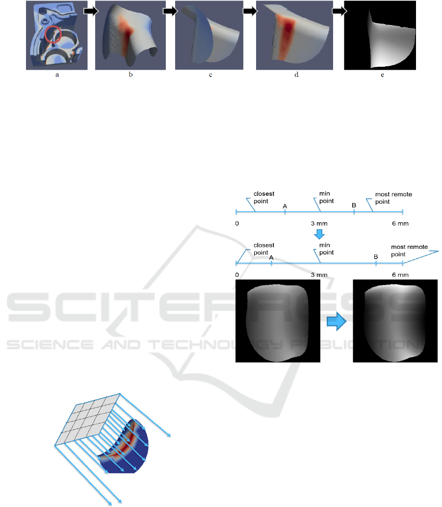
Figure 2: The process of generating depth image of 3D model.
of the generated images was increased. However, it
was done in such a way that the analysed point always
coloured as 127 (“located” 3 mm away from the grid).
At the same time closer and further parts are
“zoomed” proportionally to the closest and furthers
points (fig. 4). We understand that the procedure of
increasing contrast produces a risk of losing
information about curvature, however, this was not a
case for the considered training set.
Resnet18 was chosen as a classification model.
Resnet18 is a 18 layers deep residual CNN for image
classification (He et al., 2016). Experimentation
showed that usage of pre-trained network did not give
any advantage during training, so the network with
randomly initialised weights was used. The following
training parameters were applied for training:
Additional linear layer was added with sigmoid
output at the network output for binary
classification;
Error function: cross entropy;
Used augmentations (for training set only) are
horizontal flip and 15 rotations by 22,5 degrees
(31 augmentations for each sample);
Learning rate 1.0e-6 (no learning rate degrading);
Batch size: 32.
Figure 3: Measuring distance between a surface and 3D
object.
The network was implemented in TorchVision
library (Facebook Inc., 2020) ver. 0.6.0. One training
procedure (1 fold and 50 epochs) on the Intel Xeon
server with Nvidia Geforce 2080 RTX GPU took
about 35 minutes. The training results are presented
in fig. 5-7.
For the comparison with other techniques, the
following numbers of epochs have been chosen for
each of the radius that let one to avoid overfitting:
2 mm – 20 epochs (no more significant
improvement), 3 mm – 14 epochs (further training
causes overfitting), and 4 mm – 8 epochs (further
training causes overfitting).
Figure 4: Increasing the contrast of depth images.
One can see that classification of samples with the
radius of 2 mm produces the best results, however,
there is a concern that in the future analysing such
small fragments of the parts can produce false results.
On the other side, fragments with the radius of 4
mm are not classified well and the model becomes
overfitted already after 10 epochs, with the loss
function values being higher than those for smaller
fragments. As a result, for future research the
classification of fragments with radiuses of 2 and 3
mm were selected.
6 3D CNN-BASED
CLASSIFICATION OF
VOXELIZED MODELS
The third implemented model is an adaptation of a 3D
CNN to the reliability classification problem. The
IN4PL 2020 - International Conference on Innovative Intelligent Industrial Production and Logistics
18
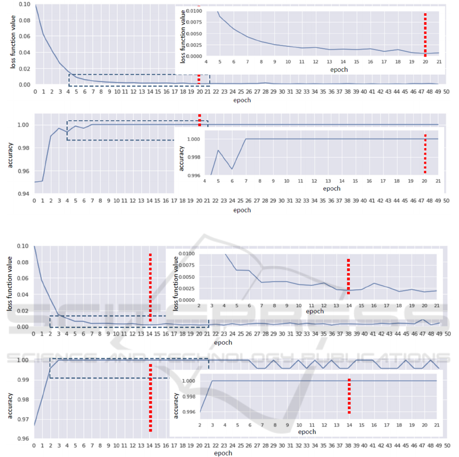
Figure 5: Training results of Resnet18-based depth image classification of 2 mm radius fragments.
Figure 6: Training results of Resnet18-based depth image classification of 3 mm radius fragments.
rationale is that two-dimensional representation (even
with the depth map) misses some details of the part
(e.g., it cannot distinguish between solid and hollow
parts), and 3D model makes the difference between
the inside and outside of the part more obvious. It is
self-evident, that 3D representation contains much
more detail about an object. The reason why neural
networks for processing 3D data receive relatively less
attention is that in most cases there are just no accurate
3D data. For example, in object detection problem, 3D
representation typically should be constructed from 2D
data or LiDAR data and this reconstruction is a
problem itself. However, in the area of manufacturing
(CAD/CAM systems) precise 3D models are available,
which makes 3D neural networks (and 3D CNN, in
particular) a reasonable choice.
We have adapted VoxNet architecture described in
(Maturana & Scherer, 2015). Original VoxNet is
designed for object recognition problem and has
softmax output layer (with the number of output units
equal to the number of classes of objects). As
reliability classification is binary classification
problem, we changed the softmax output layer to a
dense layer consisting of one unit with sigmoid
activation function. We used the same input size as
the
original
model:
32x32x32
(fig.
8). Overall,
the
Validating Results of 3D Finite Element Simulation for Mechanical Stress Evaluation using Machine Learning Techniques
19
Figure 7: Training results of Resnet18-based depth image classification of 4 mm radius fragments.
Figure 8: Example of a voxelized neighbourhood of a SF
minimum.
adapted VoxNet implementation has the following
structure:
1.
3D convolution layer with filter size 5, strides 2,
normal padding and Leaky ReLU activation
function with alpha 0.1.
2. 3D convolution layer with filter size 3, strides 1,
normal padding and Leaky ReLU activation
function with alpha 0.1.
3. 3D max pooling layer with pool size 2 and strides
2.
4. Reshape to flat vector (of size 6*6*6*32).
5. Dense layer with 128 units and ReLU activation.
6. Dense output unit with sigmoid activation.
The network is trained with the Adam algorithm
for minimization of binary cross-entropy as a loss
function.
The data preparation procedure is the following.
The part model is rotated to align the direction of the
normal at the point of the examined SF minimum with
Z axis. Then, the neighbourhood of the examined SF
minimum node is transformed into a voxel model
32x32x32 so that the minimum SF point corresponds
to the centre of the cube (voxel with coordinates [17;
17; 17]). The size of each voxel is 0.1 mm
3
, therefore,
a whole voxelized neighbourhood has dimensions
3.2x3.2x3.2 mm. An example of a pre-processed
network input is shown in fig. 8. While the position
of the normal at SF minimum is determined by the
pre-processing step, the part may still be rotated
around Z axis resulting in different models and
potentially different results. To achieve the invariance
to this rotations, we used an augmentation scheme,
according during the training voxelization of 16
rotations of each model around Z axis were
considered, and for each rotation, also one flipping.
Therefore, each SF minimum point results in 32
training samples.
7 EVALUATION AND
COMPARISON
The dataset contains 814 mesh models (samples) with
SF assigned to each vertex of the mesh. Sample label
in the dataset is determined by the expert
classification of the node with the lowest SF (global
minimum) reliability. The dataset contains 304
samples with reliable global minimum and 510
samples with non-reliable global minimum.
IN4PL 2020 - International Conference on Innovative Intelligent Industrial Production and Logistics
20

To evaluate the classification algorithms, the k-
fold cross-validation procedure has been carried out.
In accordance with this procedure, the data set is
divided into k subsets of approximately equal size,
and k experiments are performed so that each of the k
subsets is used once as the test set and the other k-1
subsets are put together to form the train set. In our
case the dataset has been split into 5 folds (k=5). The
resulting train and test sets are presented in Table 3.
During splitting the dataset, the following
consideration was taken into account. Not all models
of the dataset correspond to different components but
to result of a different simulations, i.e. a different
mechanical load case. As a result, some samples may
correspond to the same component but have different
SF values and different vertices with minimal SFs.
This fact was taken into account during splitting. It
turned out that different simulations of the same part
tend to place minimum SF to similar locations of the
part. Therefore, to prevent overfitting to a particular
part, the folds were created in such a way, that the
same part does not present both in the train and test
sets (sometimes, this is referred to as “group K-fold
validation”; in this case, the group is interpreted as
simulation results of one component).
The described above algorithms have been
evaluated on the same set of folds. They include
(1) CatBoost with all features, (2) CatBoost with top
10 features, (3-5) Resnet18 for neighborhoods with
radiuses of 2 mm, 3 mm, and 4 mm, and (6) VoxNet.
We have also added the logistic regression as a base
classification model for the comparison.
To evaluate the algorithms two types of criteria
were considered: performance, measured by training
and prediction times; and prediction quality,
measured by accuracy. However, it turned out that the
accuracy values were quite high, so the absolute
number of misclassified samples was also considered
(it does not provide additional information compared
to the accuracy, but slightly easier to read and
interpret). The results of the evaluation are shown in
Table 4.
It can be seen, that all the models achieve quite
good results in terms of accuracy. Logistic regression
has a significant advantage in training time over the
other models, but has the lowest accuracy. Taking
into account, that training is not so frequent operation
in the intended use cases of the model, and training
times of deep learning models are also reasonable,
this advantage is not very important. None of the
explored feature-based models were able to achieve
perfect classification, which is most likely related to
the fact that proposed features didn’t describe
significant aspects of the SF minimum
neighbourhood necessary for such classification.
Among
the deep learning-based models, 3D CNN
Table 3: Distribution of samples for folds used in the experiment.
Fold
Train set Test set
“Reliable”
samples
“Unreliable”
samples
Total
“Reliable”
samples
“Unreliable”
samples
Total
1 258 391 649 46 119 165
2 212 437 649 92 73 165
3 246 405 651 58 105 163
4 252 401 653 52 109 161
5 248 406 654 56 104 160
Table 4: Comparison of approaches to Validating Results of 3D Finite Element Simulation.
Classification
approach
Errors on fold
Mean training time, s
Mean prediction
time, s
Mean accuracy
Mean # of
errors
1 2 3 4 5
Logistic regression 2 1 0 0 10 0.017 0.006 0.984 2.6
CatBoost 0 4 0 0 0 1.58 0.008 0.995 0.8
CatBoost
(10 features)
0 2 2 2 0 0.988 0.007 0.993 1.2
Resnet18 (radius
2)
0 0 0 0 0
800 (GPU, 20
epochs)
0.036
(no GPU)
1 0
Resnet18 (radius
3)
0 0 0 0 0
560 (GPU, 14
epochs)
0.036
(no GPU)
1 0
Resnet18 (radius
4)
0 0 0 0 0 320 (GPU, 8 epochs)
0.036
(no GPU)
1 0
VoxNet 0 0 0 0 0 9.6 (GPU, 3 epochs) 0.161 1 0
Validating Results of 3D Finite Element Simulation for Mechanical Stress Evaluation using Machine Learning Techniques
21

VoxNet can be considered the best, as it achieves
perfect classification of the provided dataset and has
significantly lower training time than other models. It
supports the initial intuition that 3D CNN should be a
reasonable choice as they fully exploit the 3D
structure of analysed components.
Based on the results, it was decided that further
research should focus on the Resnet18 models for the
radius of 2 and 3 mm and the VoxNet model.
8 CONCLUSIONS
The paper is aimed at application of AI techniques to
reliability evaluation of 3D simulation results
produced via 3D finite element simulation. It was
found that such classification is possible by various
3D model classification techniques, and some of them
produce perfectly accurate results.
Among the machine learning approach, relying on
geometrical features, 2D depth image classification
via Resnet18, and VoxNet-based classification of
voxelized models, the latter two were selected for
further analysis.
Future research is planned to be aimed for two
major aspects. First, currently only global SF minima
were classified, whereas in reality, local minima need
to be classified as well.
Second, absolute sizes of components (and
component fragments) were used for classification.
However, there can be components with significantly
different sizes and the appropriate sample radius may
differ from the findings in this paper. Approaches to
either scale models or choose the fragments according
to the number of included vertices need to be studied,
which might be more generic for varying component
sizes.
ACKNOWLEDGEMENTS
The paper is due to collaboration between SPIIRAS
and Festo SE & Co. KG. The state-of-the-art analysis
(sec. 3) is due to the grant of the Government of
Russian Federation (grant 08-08). The CNN-based
classification (sec. 5) is partially due to the State
Research, project number 0073-2019-0005.
REFERENCES
Ahmed, E., Saint, A., Shabayek, A. E. R., Cherenkova, K.,
Das, R., Gusev, G., Aouada, D., & Ottersten, B. (2018).
A survey on Deep Learning Advances on Different 3D
Data Representations. http://arxiv.org/abs/1808.01462
Altmann, A., Toloşi, L., Sander, O., & Lengauer, T. (2010).
Permutation importance: a corrected feature importance
measure. Bioinformatics, 26(10), 1340–1347.
https://doi.org/10.1093/bioinformatics/btq134
Charles, R. Q., Su, H., Kaichun, M., & Guibas, L. J. (2017).
PointNet: Deep Learning on Point Sets for 3D
Classification and Segmentation. 2017 IEEE
Conference on Computer Vision and Pattern
Recognition (CVPR), 77–85.
https://doi.org/10.1109/CVPR.2017.16
Cohen-Steiner, D., & Morvan, J.-M. (2003). Restricted
delaunay triangulations and normal cycle. Proceedings
of the Nineteenth Conference on Computational
Geometry - SCG ’03, 312.
https://doi.org/10.1145/777792.777839
Dawson-Haggerty et al. (n.d.). trimesh.
Deng, X., Zheng, Y., Xu, Y., Xi, X., Li, N., & Yin, Y.
(2018). Graph cut based automatic aorta segmentation
with an adaptive smoothness constraint in 3D
abdominal CT images. Neurocomputing, 310, 46–58.
https://doi.org/10.1016/j.neucom.2018.05.019
Facebook Inc. (2020). PyTorch. https://pytorch.org/
Feng, J., Wang, Y., & Chang, S.-F. (2016). 3D shape
retrieval using a single depth image from low-cost
sensors. 2016 IEEE Winter Conference on Applications
of Computer Vision (WACV), 1–9.
https://doi.org/10.1109/WACV.2016.7477652
Grellier, O. (2018). Feature Selection With Null
Importances.
Hanocka, R., Hertz, A., Fish, N., Giryes, R., Fleishman, S.,
& Cohen-Or, D. (2019). MeshCNN: A Network with an
Edge. ACM Transactions on Graphics, 38(4), 1–12.
https://doi.org/10.1145/3306346.3322959
He, K., Zhang, X., Ren, S., & Sun, J. (2016). Deep Residual
Learning for Image Recognition. 2016 IEEE
Conference on Computer Vision and Pattern
Recognition (CVPR), 770–778.
https://doi.org/10.1109/CVPR.2016.90
Ioannidou, A., Chatzilari, E., Nikolopoulos, S., &
Kompatsiaris, I. (2017). Deep Learning Advances in
Computer Vision with 3D Data. ACM Computing
Surveys, 50(2), 1–38. https://doi.org/10.1145/3042064
Kitware Inc. (2005). File Formats for VTK Version 4.2.
https://vtk.org/wp-content/uploads/2015/04/file-
formats.pdf
Lu, X., Xie, Q., Zha, Y., & Wang, D. (2018). Fully
automatic liver segmentation combining multi-
dimensional graph cut with shape information in 3D CT
images. Scientific Reports, 8(1), 10700.
https://doi.org/10.1038/s41598-018-28787-y
Ma, L., Sacks, R., Kattel, U., & Bloch, T. (2018). 3D Object
Classification Using Geometric Features and Pairwise
Relationships. Computer-Aided Civil and
Infrastructure Engineering, 33(2), 152–164.
https://doi.org/10.1111/mice.12336
Ma, Z., Wu, X., Song, Q., Luo, Y., Wang, Y., & Zhou, J.
(2018). Automated nasopharyngeal carcinoma
segmentation in magnetic resonance images by
IN4PL 2020 - International Conference on Innovative Intelligent Industrial Production and Logistics
22

combination of convolutional neural networks and
graph cut. Experimental and Therapeutic Medicine.
https://doi.org/10.3892/etm.2018.6478
Maturana, D., & Scherer, S. (2015). VoxNet: A 3D
Convolutional Neural Network for real-time object
recognition. 2015 IEEE/RSJ International Conference
on Intelligent Robots and Systems (IROS), 922–928.
https://doi.org/10.1109/IROS.2015.7353481
Qiao, K., Zeng, L., Chen, J., Hai, J., & Yan, B. (2018). Wire
segmentation for printed circuit board using deep
convolutional neural network and graph cut model. IET
Image Processing, 12(5), 793–800.
https://doi.org/10.1049/iet-ipr.2017.1208
Reddy, J. N. (2009). An Introduction to the Finite Element
Method (3rd ed.). McGraw-Hill.
Schwarz, M., Schulz, H., & Behnke, S. (2015). RGB-D
object recognition and pose estimation based on pre-
trained convolutional neural network features. 2015
IEEE International Conference on Robotics and
Automation (ICRA), 1329–1335.
https://doi.org/10.1109/ICRA.2015.7139363
Su, H., Maji, S., Kalogerakis, E., & Learned-Miller, E.
(2015). Multi-view Convolutional Neural Networks for
3D Shape Recognition. 2015 IEEE International
Conference on Computer Vision (ICCV), 945–953.
https://doi.org/10.1109/ICCV.2015.114
Wahl, E., Hillenbrand, U., & Hirzinger, G. (2003). Surflet-
pair-relation histograms: a statistical 3D-shape
representation for rapid classification. Fourth
International Conference on 3-D Digital Imaging and
Modeling, 2003. 3DIM 2003. Proceedings., 474–481.
https://doi.org/10.1109/IM.2003.1240284
Wang, Y., Sun, Y., Liu, Z., Sarma, S. E., Bronstein, M. M.,
& Solomon, J. M. (2019). Dynamic Graph CNN for
Learning on Point Clouds. ACM Transactions on
Graphics, 38(5), 1–12.
https://doi.org/10.1145/3326362
Wang, Y. Y., & Li, J. (2008). Featureselection ability of
the decisiontree algorithm and the impact of feature
selection/extraction on decisiontree results based on
hyperspectral data. International Journal of Remote
Sensing, 29(10), 2993–3010.
https://doi.org/10.1080/01431160701442070
Yandex. (2020a). CatBoost - Feature Importance.
Yandex. (2020b). CatBoost - open-source gradient
boosting library.
Yavartanoo, M., Kim, E. Y., & Lee, K. M. (2019). SPNet:
Deep 3D Object Classification and Retrieval Using
Stereographic Projection. Computer Vision – ACCV
2018. Lecture Notes in Computer Science, 11365, 691–
706. https://doi.org/10.1007/978-3-030-20873-8_44
Zhou, H.-Y., Liu, A.-A., Nie, W.-Z., & Nie, J. (2020).
Multi-View Saliency Guided Deep Neural Network for
3-D Object Retrieval and Classification. IEEE
Transactions on Multimedia
, 22(6), 1496–1506.
https://doi.org/10.1109/TMM.2019.2943740
Validating Results of 3D Finite Element Simulation for Mechanical Stress Evaluation using Machine Learning Techniques
23
