Detection of Ball Spin Direction using Hitting Sound in Tennis

Naoki Yamamoto

1 a

, Kenji Nishida

1 b

, Katsutoshi Itoyama

1 c

and Kazuhiro Nakadai

1,2 d

School of Engineering, Tokyo Institute of Technology, Tokyo, Japan

Honda Research Institute Japan Co., Ltd., Saitama, Japan

Keywords:

Sports Science, Tennis, Acoustic Analysis of Impact, Ball Spin Detection.

Abstract:

This paper describes the detection of rotation direction using the hitting sound of tennis balls. Since each

ball rotation direction has a slightly different rotation direction and trajectory, there should be a difference

in the hitting sound. To distinguish the characteristics of ball rotation direction, a database was constructed

that combines the hitting sound recorded experimentally with ball rotation direction. Since it is difﬁcult

to distinguish audible differences in hitting sounds by ear, it is necessary to identify them using measuring

instruments. For this purpose, after extracting the amplitude spectrum by fast Fourier transform of the shot

sound, the entire data was normalized and classiﬁed by a support vector machine. As a result of evaluating this

method, a high accuracy was obtained in identifying the sound associated with slice among other hit sounds.

The proposed method also evaluated the ball hit sound from a YouTube video in an unknown environment and

achieved a perfectly correct identiﬁcation of spin and slice.

1 INTRODUCTION

In recent years, there has been a growing movement

worldwide to introduce science and technology

into sports. Smart courts (SecondSpetrum, 2020;

Playsight, 2020), which have multiple cameras that

can track the movement of players and balls using

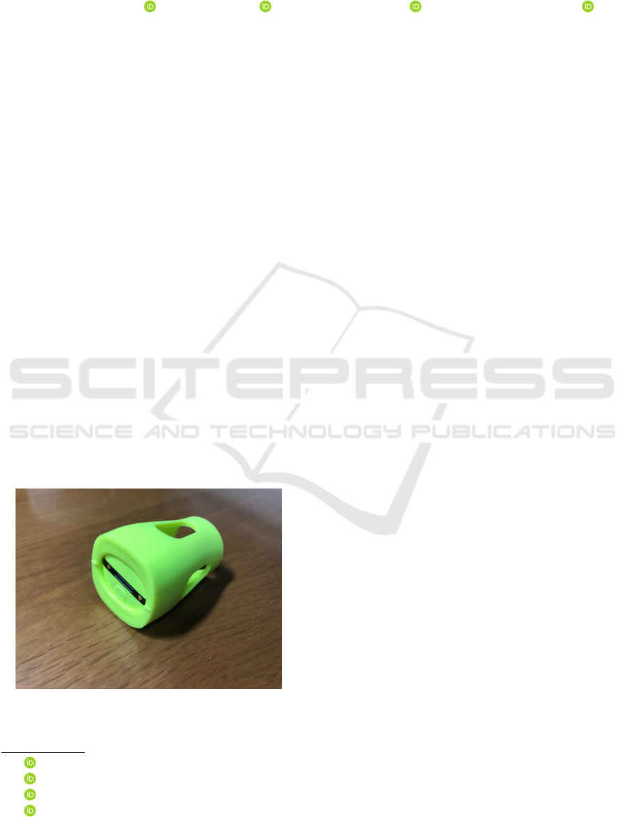
Figure 1: Smartsensor can be attached to the grip end of

the racket and can measure the rotation direction, speed,

rotational speed, etc. of the stroke.

https://orcid.org/0000-0001-7367-4725

https://orcid.org/0000-0003-4214-4005

https://orcid.org/0000-0002-7098-3896

https://orcid.org/0000-0002-6134-4558

computer vision technology, are utilized in various

sports such as football, basketball, and so on (Seo

et al., 2018). The smart court system developed to

improve the accuracy of umpire decisions in tennis in-

troduced “Hawkeye” which includes eight super high-

speed cameras to specify the trajectory and landing

point of the ball (Baodon, 2014) to inform umpires in

professional matches and to smoothly advance games.

However, smart courts require large systems to be

installed and their cost prohibit personal use. Form

(pose) analysis is an important issue in computer vi-

sion for sports in which many studies have been re-

ported (Cust et al., 2019; Appelbaum and Erickson,

2018; Okamoto et al., 2015; Cao et al., 2019). Such

studies have achieved signiﬁcant progress in many

sports, but one important issue has not been studied

well in ball games – the detection of the spin (or rota-

tion) direction of balls.

The trajectory of a ball is greatly affected by its

rotation, so players need to be able to detect the rota-

tion direction to predict the ball trajectory. In tennis

especially, players need to be able to perform balls

with various rotation and also identify the rotation di-

rection of the opponents’ balls. A smart tennis sen-

sor (Zepp, 2020) has been developed to measure ball

speed, rotation direction and revolution using an ac-

celerometer and three-axis gyro-sensor, which is usu-

ally attached to the grip-end of the racket (Figure 1).

Yamamoto, N., Nishida, K., Itoyama, K. and Nakadai, K.

Detection of Ball Spin Direction using Hitting Sound in Tennis.

DOI: 10.5220/0010107600300037

In Proceedings of the 8th International Conference on Sport Sciences Research and Technology Support (icSPORTS 2020), pages 30-37

ISBN: 978-989-758-481-7

Players can learn to hit various rotation directions by

using smart tennis sensors, but they do not provide in-

formation about the opponent’s treatment of the ball.

Ball rotation can be detected using a high-speed and

high-resolution camera, but since tennis is a sport in

which the balls travel fast in a short period of time,

and are hit at various places in the court, a precise

tracking system is required in addition.

Since tennis players are known to make decisions

based on the hitting sound of the opponent, in this

study, we focused on the hitting sound. Although

some previous studies focused on the hitting sound

of tennis balls during play, they paid attention only to

ball speed (Zhang et al., 2017). In depth research on

hitting sound and ball rotation direction has not been

previously conducted. However, Canal-Bruland et al

asked subjects to watch a professional tennis match

on video and predict the trajectory of the ball at that

time (Canal-Bruland, 2018). As a result, it was shown

that the hitting sound could be an important factor in

predicting the ball trajectory. In predicting the tra-

jectory of a ball, three types of the rotation direc-

tion, namely spin, ﬂat, and slice form the basis of ball

movement pattern. By recognizing rotation direction,

a rough trajectory of the ball can be predicted, and

player performance can improve as prediction accu-

racy improves.

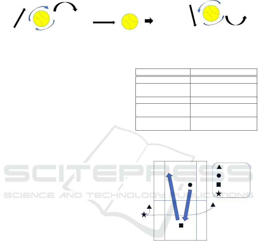
A spin hit happens when the head of the racket is

rotated over the top of the ball during a hit causing a

tangential velocity of the top of the ball in the same di-

rection as the ball’s trajectory resulting in lower drag

force at the bottom of the ball so it falls downwards

(Figure 2a). A ﬂat hit ball does not spin to any sig-

niﬁcant degree so does not veer from the direction in

which it is hit (Figure 2b). A slice hit, contrary to

spin, happens when a player angles the racket back

and slides it underneath the ball when hitting which

makes it veer upwards. The tangential velocity of the

top of the ball is in the opposite direction of the tra-

jectory of the ball, so the force of this hit tends to

be weaker than spin or ﬂat. Players may also make

the ball deﬂect left or right by corresponding rota-

tions (Figure 2c). To validate the proposed method,

a set of tests was, performed to obtain necessary ball

hitting sound data. Then, a identiﬁable data set was

constructed using a developed identiﬁer. Thereafter,

accuracy of the identiﬁer was evaluated. Finally, we

sampled ball hitting sounds from YouTube and ap-

plied the identiﬁer to observe the percentage of cor-

rect answers.

Following, Section 2 describes related research,

Section 3 describes the database constructed, Section

4 proposes a method for processing the data, and Sec-

tion 5 describes the results and considerations of eval-

uation experiments using the proposed method.

2 RELATED RESEARCH

To improve player performance in tennis, Asano et al.

attached markers to a ball and used high-speed cam-

eras to determine the rotation angle and number of ro-

tations for each of three axes. Three-dimensional lo-

cation of the ball center was obtained from the camera

parameters with two cameras, and the ball trajectory

was estimated.

Elsewhere, research has focused on the sound of

hitting balls in sound table tennis. A game was de-

signed for blind people with a rule that if no returned

ball hitting sound was heard, it was a foul. Because

the judge only relied on hearing, application of the

rule was ambiguous. Kogusuri et al. aimed to clarify

this rule (Kogusuri et al., 2008). In that research, they

propose a technique to determine a hit by focusing on

frequency domain components by recording the hit

sound with a digital audio tape recorder via a noise

meter, applying wavelet transform analysis, and us-

ing the hit sound. Similar concept was used aimed at

improving the player performance in other ball sports

studies focusing on the hitting sound. Although the

effect of ball hitting sound on performance has been

studied, waveform characteristics of the hitting sound

have not been clariﬁed.

Therefore, Zhang et al. are conducting research of

the latent characteristics of the hitting sounds of op-

ponent players (Zhang et al., 2017). In their study,

the sound of hitting a service ball was extracted from

the deuce side and the advantage side in 15 examples

each, and the characteristics were compared by over-

lapping the time domain waveforms. Speciﬁcally, a

television image was recorded and its sound was ex-

tracted, the ﬁrst peak of each sound waveform was

overlapped and compared for each player, and the

sound characteristics of each player were detected

from the average amplitude of the ﬁrst peak and the

arrival time between the ﬁrst peak and the last peak.

It is deﬁned that a sample point has a peak when it

has a greater value than two adjacent sample points

and a certain threshold. It is how to ﬁnd peaks. They

reported a correlation between ball speed and hitting

sound magnitude, but rotation direction was not men-

tioned.

Hitting sound has been studied in other sports.

However, in tennis, although some studies aimed at

improving performance focused on the sound of hit-

ting balls, no study has been conducted to determine

ball rotation from the sound of hitting balls as far as

we know. In this study, we focused on ball hitting

Detection of Ball Spin Direction using Hitting Sound in Tennis

Direction of Travel

Direction of Racket Swing

Direction of Rotation

(a) Spin rotation direction.

Direction of Travel

Direction of Racket Swing

(b) Flat rotation direction.

Direction of Travel

Direction of Racket Swing

Direction of Rotation

Figure 2: Three types of rotational directions.

sound to describe and identify rotation direction.

3 METHODS AND

CONSTRUCTION OF BALL

HITTING SOUND DATABASE

This section describes experiments to construct a hit-

ting sound database, and processing algorithm to con-

struct a hitting sound pattern database from collected

sound data.

3.1 Recording Exercise

The purpose of this exercise was to record spin, ﬂat,

and slice shot sounds and create a basic pattern data

set to identify rotation directions. The recording was

performed under the following conditions.

• Date & Time: 2019/12/10 11:00-13:00

• Place: Ninomiya Park Tennis Court (hard court,

outdoor), Tsukuba City, Japan

• Weather: Sunny & almost no wind

• Hitter: A male, 15 years of tennis experience

Figure 3 illustrates the experimental setting, and

Table 1 shows speciﬁcations of the equipment used in

the recording. The hitting procedure is controlled to

maintain the quality of recorded sounds as follows:

1. A ball person throws a ball for a hitter.

2. The hitter hits the ball with a certain direction and

force which is decided by the hitter.

3. The hitter tells a recorder the rotation direction

(and force) that the hitter decided.

In total, 92 trials were performed.

3.2 Ball Hitting Sound Database

Construction

For each recorded sound, a 50 ms clip was extracted

so that each clip can include the moment of impact.

This was manually done for all 92 recorded sound

Table 1: Equipment used in the recording.

Equipment Description

Microphone type TAMAGO-03

Microphone position 2 near the pillars con-

nected straight to PC

Tennis ball 20 new balls

Racket SRIXON REVO CV3.0

(SR21802)

PC 16 kHz and 16-bit record-

ing

data using Audacity. We, thus, collected a ball hit-

ting pattern dataset consisting of 92 sound clips and

the corresponding rotation direction.

Ball trajectory

USB cable

Microphone

Ball person

Hitter

Figure 3: Experimental setup. A ball person throws a ball,

and a hitter hits the ball. Arrows show a typical trajectory

of the ball for a single trial.

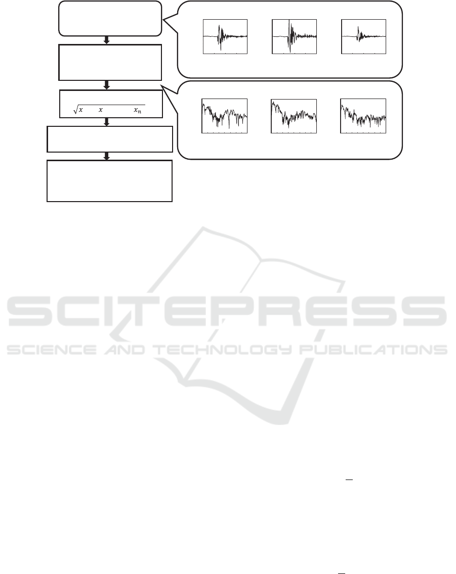
4 PROPOSED METHOD

This section explains the proposed method to identify

rotation direction from hitting sound. The proposed

method uses frequency analysis, data normalization,

dimensionality reduction, and 2-class SVM to clas-

sify the ball rotation (Figure 4).

icSPORTS 2020 - 8th International Conference on Sport Sciences Research and Technology Support

slice

Input: Amplitude spectrum (91dim)

Output: Ball rotation (spin, flat, slice)

Normalization

+ ⋯ +

Constructed dataset

spin

amplitude spectrum

spin

flat

slice

Frequency analysis

Window length: 800

FFTsample point: 1024

flat

Recorded hitting sound

Sampling frequency: 16kHz

Length of sound: 50ms

Support vector machine

Principal component analysis

0 200 400 600 800

Time (sample)

-0.5

-0.4

-0.3

-0.2

-0.1

0.1

0.2

0.3

0.4

0.5

Amplitude

0 200 400 600 800

Time (sample)

-0.5

-0.4

-0.3

-0.2

-0.1

0.1

0.2

0.3

0.4

0.5

Amplitude

0 200 400 600 800

Time (sample)

-0.5

-0.4

-0.3

-0.2

-0.1

0.1

0.2

0.3

0.4

0.5

Amplitude

0 1 2 3 4 5 6 7 8

Frequency (kHz)

-50

-40

-30

-20

-10

Amplitude (dB)

0 1 2 3 4 5 6 7 8

Frequency (kHz)

-50

-40

-30

-20

-10

Amplitude (dB)

0 1 2 3 4 5 6 7 8

Frequency (kHz)

-50

-40

-30

-20

-10

Amplitude (dB)

513dimЍ 91dim

Figure 4: Flowchart of the proposed method.

4.1 Frequency Analysis

The input sound pattern is assumed to have 50 ms du-

ration including the impact of hitting as described in

Section 3. Fourier transform is performed for the in-

put signal. Fourier transform is a frequency analysis

method used to decompose a complex sound into its

constituent parts, and there is an algorithm to greatly

increase the speed of the discrete Fourier transform,

which is called fast Fourier transform (FFT). FFT is

beneﬁcial when dealing with a large amount of data,

and thus we decided to use FFT with a rectangular

window for frequency analysis. In the present case,

the number of data sets to be processed was 92. Since

the sampling frequency was set at 16 kHz and the time

component of clipped signals was 50 ms, the length

of the signal was 800 samples. For FFT, the win-

dow length of 1024 samples with zero padding was

adopted. When FFT is applied, the real part of the

frequency-amplitude diagram is line-symmetric, the

imaginary part is point-symmetric, that is, it is con-

jugate, and the amplitude spectrum is line-symmetric.

Therefore, the frequency component of interest at this

time was 0–8 kHz (Nyquist frequency). Thus, the

number of dimensions of the data to be treated this

time was 513 dimensions. The analysis was per-

formed using MATLAB.

4.2 Data Normalization

Normalization was performed to prevent variation due

to the difference of the impacted position for each

data.

4.3 Dimensionality Reduction with

Principal Component Analysis

Since only 92 samples with a 513 dimensional fea-

ture representation for each impact sound were ob-

tained, the training samples should be mapped to the

lower dimensional feature space to ensure good gen-

eralization performance. Principal component anal-

ysis (PCA) (Diamantaras and Kung, 1998) estimates

principal components of a dataset, where a principal

component with a larger score gives better representa-

tion of the dataset. By selecting principal components

with larger scores, the dataset is well represented with

a lower dimensional feature space. Therefore, we

applied the Principal Component Analysis (PCA) to

our impact sound data. The procedure of PCA is de-

scribed as follows. Let x

(i = 1,..., N) represent the

i-th D-dimensional data. The DC offset is ﬁrst re-

moved by,

= x

−

∑

j=1

). (1)

DC offset is the addition of a Direct Current compo-

nent to a device’s performance and the effect of sur-

rounding electrical inﬂuences that causes it to deviate

from 0V.

The covariance matrix of X is, then, calculated as,

∑

i=1

. (2)

Eigenvalue decomposition is performed for the ob-

tained covariance matrix X by,

U = UΛ, (U

U = I), (3)

Detection of Ball Spin Direction using Hitting Sound in Tennis

0 100 200 300 400 500

Feature dimention

0.1

0.2

0.3

0.4

0.5

0.6

0.7

0.8

0.9

Contribution rate

Figure 5: Cumulative contribution rates of PCA for the con-

structed database. The horizontal axis is the dimension of

rotation direction and the vertical axis is the cumulative con-

tribution rate at the selected feature dimension.

where U is the square D×D matrix whose i-th column

is the eigenvector, and Λ is the diagonal matrix whose

diagonal elements are the corresponding eigenvalues.

Figure 5 shows a cumulative contribution rate for

ﬁrst 91 principal components in the descending order.

Since the cumulative contribution rate reached 1 with

the 91 principal components, the number of dimen-

sions was set to 91 in the feature vector for identiﬁca-

tion. Note that due to rank deﬁcient, the rate reached

1 with 91 principal components for 92 samples. In

Figure 5, the rate also reached 0.7 with 20 principal

components, and we will also verify a lower feature

such as a 20-dimensional feature in the evaluation.

4.4 SVM

The proposed method performs two-class classiﬁca-

tion. For example, when a target is spin, the iden-

tiﬁcation is to discriminate whether the sound is for

spin or not. This means that three types of two-class

identiﬁcation, that is, for spin, ﬂat, and slice were per-

formed.

For the low dimensional input vector, s, obtained

by PCA, we ﬁrst introduce a general classiﬁcation

function, y, deﬁned as,

y = sign

(

s − h

)

, (4)

where w indicates a weight vector for the input and

h is a threshold. Function sign(u) is a sign func-

tion, which outputs 1 when u > 0 and outputs -1 when

u ≤ 0. In other words, Eq. (4) separates a space rep-

resented by s into two sub-spaces using a separating

hyperplane deﬁned by w. An SVM (Scholkopf et al.,

1999; Vapnik, 1998) is a method to determine the sep-

arating hyperplane that maximizes the distance (mar-

gin) between the separating hyperplane and the near-

est sample. However, in a conventional SVM, all in-

put samples should be linear separable, which is de-

Table 2: The number of data and class weight.

Identiﬁer spin ﬂat slice

positive sample 46 16 30

negative sample 46 76 62

1 5 2

ﬁned by,

− h) ·t

≥ 1, i = 1,...,N, (5)

where t

shows the correct class label (1 or −1) for s

stands for the i-th input vector.

This means that the samples are separated by two

hyperplanes such as

H1 : w

− h = 1, (6)

H2 : w

− h = −1, (7)

and there are no samples between these two hyper-

planes. The distance between the separating hyper-

plane and each of these hyperplanes is deﬁned as

1/∥w∥.

To relax a linear separable constraint, a soft-

margin is introduced to SVM, which allows training

samples between H1 and H2. For this, a distance pa-

rameter ξ

for s

is introduced. It is deﬁned for the i-th

sample with t

= 1 as,

{

−w

+ h + 1 (w

− h < 1)

0 (otherwise)

(8)

It is also deﬁned for the i-th sample with t

= −1 as,

{

− h + 1 (w

− h > −1)

0 (otherwise)

(9)

The soft-margin SVM is, then, deﬁned as an opti-

mization problem to minimize a cost function deﬁned

by,

L(w,ξ) =

∥w∥

∑

i=1

(10)

subject to

≥ 0, t

· (w

− h) ≥ 1 − ξ

, (i = 1, . . .,N), (11)

where ξ = {ξ

|i = 1,··· ,N}. C stands for a cost pa-

rameter for ξ. q

is a weight for the i-th sample deﬁned

by,

{

1 s

∈ C

|x ∈ C

|/|x ∈ C

| s

∈ C

(12)

where C

and C

indicate the smaller and the larger

class, respectively.

Mentioned above, there are three types of identi-

ﬁers such like Table 2.

icSPORTS 2020 - 8th International Conference on Sport Sciences Research and Technology Support

Solving this problem with an optimal solution α,

the classiﬁcation function can be redeﬁned as

y = sign (w

s − h)

= sign (

∑

i∈S

s − h). (13)

where S stands for the indices of the support vectors.

The samples are grouped with α

; a sample s

is classi-

ﬁed correctly when α

= 0, when 0 < α

< C the sam-

ple s

is also classiﬁed correctly and it locates on the

hyperplane H1 (or H2) as a support-vector, if α

= C

the sample s

becomes a support-vector but it locates

between H1 and H2 with ξ ̸= 0.

The recorded signal data was fed into the support

vector machine (SVM). The number of data examples

was 92. Therefore, a method called the Leave One

Out Cross-Validation (LOOCV), which splits up the

sample into two categories: validation data, made up

of one data from the sample, and training data, made

up of the rest of the data in the sample, was used to ex-

amine the data. The sample was given a class weight,

and the classiﬁcation was carried out accordingly. Us-

ing LOOCV is advantageous as it prevents overﬁtting

for few data, as observations are made on N-1 sam-

ples.

The present method identiﬁes one rotation direc-

tion and others, such like spin and not spin (ﬂat and

slice). Then, using the hyperparameter optimization

function in MATLAB, the parameter of the soft mar-

gin in which the accuracy was at maximum, was set.

5 EVALUATION

The proposed method is validated with the con-

structed ball hitting sound database and sound clips

selected from YouTube videos.

5.1 Identiﬁcation with Recorded Ball

Hitting Sound Database

Each recorded sound clip was fed into the support

vector machine (SVM) as an input. The data set was

as small as 92, and the evaluation was performed by

LOOCV explained in the previous section in order to

prevent over-ﬁtting and to maintain open test.

For each rotation, the hyper parameters such as a

soft margin were optimized using MATLAB to maxi-

mize the accuracy.

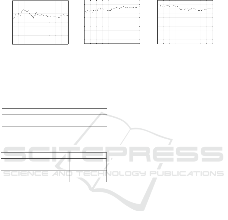
Figures 6a-6c illustrate the answer rates for identi-

ﬁcation of spin, ﬂat, and slice from the sound clip us-

ing the constructed ball hitting sound database. The

horizontal axis of each ﬁgure shows the number of

feature dimensions up to 91 in the descending order

Table 3: Confusion matrix for identiﬁcation of each ball

rotation direction. All 92 samples were identiﬁed with 91

dimensional features.

(a) Confusion matrix for identiﬁcation of spin and oth-

ers.

spin (correct) others (correct)

spin

(prediction)

35 10

others

(prediction)

11 36

(b) Confusion matrix for identiﬁcation of ﬂat and oth-

ers.

ﬂat (correct) others (correct)

ﬂat

(prediction)

11 14

others

(prediction)

5 62

others.

slice (correct) others (correct)

slice

(prediction)

27 11

others

(prediction)

3 51

of eigenvalues. It is clear that, the accuracy is over

70% for all rotation directions. It is remarkable that

the accuracy with 91 dimensions is almost identical to

that with 20 dimensions. In other words, the analysis

can be effectively and accurately performed with 20

dimensions.

Tables 3 show confusion matrices of 2-class iden-

tiﬁcation tasks with 91 feature dimensions. Each table

illustrates true-positive, true-negative, false-positive,

and false-negative scores of the identiﬁcation task. As

mentioned above, accuracy of more than 70% was ob-

tained for all three rotations , but the precision has

different characteristics. The precision of identifying

ﬂat is remarkably low like 44%, while the precision of

identifying spin and slice exceeds 70%. This is also

linked to the low F value for ﬂat.

5.2 Analysis of YouTube Clips

To apply the proposed method to YouTube clips, a

video including ball hitting sounds by a professional

tennis player were selected. The selected video is of

the world’s fourth-ranked Roger Federer practicing at

the Australian Open (hard court) in January 2020

From the video, 5 spin samples and 5 slice samples

were picked up. After that, 50 ms ball hitting sound

clips were extracted from each video in the same man-

https://youtu.be/hTn42aJIhk8

Detection of Ball Spin Direction using Hitting Sound in Tennis

0 10 20 30 40 50 60 70 80 90

Feature dimension

0.1

0.2

0.3

0.4

0.5

0.6

0.7

0.8

0.9

Accuracy

(a) Accuracy for spin.

Feature dimension

0.1

0.2

0.3

0.4

0.5

0.6

0.7

0.8

0.9

Accuracy

(b) Accuracy for ﬂat.

0 10 20 30 40 50 60 70 80 90

Feature dimension

0.1

0.2

0.3

0.4

0.5

0.6

0.7

0.8

0.9

Accuracy

Figure 6: Accuracy for each spin direcsion. The horizontal and vertical axes indicate the feature dimension and the accuracy

of two class identiﬁcation between one rotation direction and others, respectively. The accuracy is deﬁned as the number of

correctly identiﬁed sounds divided by the total number of sounds.

Table 4: Confusion matrix for hitting sound identiﬁcation.

It uses 91 feature dimensions.

(a) Identiﬁcation result of spin and others from

YouTube clips.

spin (correct) others (correct)

spin

(prediction)

5 0

others

(prediction)

0 5

(b) Identiﬁcation result of slice and others from

YouTube clips.

slice (correct) others (correct)

slice

(prediction)

5 0

others

(prediction)

0 5

ner as it was done when constructing the database.

Since the sampling rate of YouTube video sound is

44100 Hz, it was resampled at 16 kHz using the Au-

dacity. Since overtaking from experiment result, the

number of feature dimensions was set to 91.

Tables 4a and 4b show the results of identiﬁca-

tion for spin and slice, respectively. All 10 clips from

YouTube were 100% identiﬁed.

5.3 Discussion

This section discusses the results obtained from

the experiments using our own recorded sound and

YouTube clips. Not only our own recorded data but

YouTube data were successfully identiﬁed with high

accuracy. One problem is that identiﬁcation perfor-

mance for ﬂat shots was poor. This problem is con-

sidered to be caused by a small number of ﬂat data.

The training data set consists of 46 spin, 16 ﬂat and

30 slice shots. The lack of ﬂat data and data unbal-

ancing between three kinds of shots resulted in poor

precision for ﬂat data identiﬁcation. Generally speak-

ing, when focusing on an individual tennis player, it is

natural that spin and slice are easy to be distinguished

from each other, but ﬂat is difﬁcult to be detected.

This will be supported by the fact that spin and slice

are in the opposite direction of rotation, and ﬂat has

less rotation, that is, between spin and slice.

When the ﬁrst principal component is analyzed,

we found that many of determining features are re-

lated to a frequency range 250-1100 Hz. This shows

that relatively a low frequency range is needed for

good identiﬁcation although a hitting sound is impul-

sive with wide spectrum.

6 CONCLUSION

This paper describes identiﬁcation of the rotation di-

rection of tennis ball from hitting sound. We consid-

ered three class identiﬁcation, that is, spin, ﬂat, and

slice, and proposed a rotation direction identiﬁcation

method based on support vector machine and princi-

pal component analysis. We also constructed a hitting

sound database consisting of 92 hitting sounds with

labels. Using the constructed database, the accuracy

of spin identiﬁcation was over 70% for each of three

classes, although the precision of ﬂat was only about

44% due to unbalanced data and the small number of

ﬂat data. The proposed method was also applied to

10 clips selected from YouTube, and in all cases the

shots were successfully identiﬁed. Our detail analy-

sis showed that the ﬁrst principal component depends

heavily on 250-1100 Hz features, which is interesting

because hitting sound is impulsive with a lot of high

frequencies in the spectrum.

icSPORTS 2020 - 8th International Conference on Sport Sciences Research and Technology Support

7 FUTURE WORK

For YouTube, all 10 clips were successfully identi-

ﬁed, which shows that the models trained with SVM

worked properly, although the number of YouTube

clips is still small. Since the number of data is lim-

ited, we need to conﬁrm the generality using a large

amount of data. Also, the robustness of the identiﬁ-

cation should be veriﬁed, because other noise sources

will be mixed into the input sound, and the distance

between a microphone and a sound source can not

be well controlled in practice, and the deference of

experiment place and weather. Future work also in-

cludes an extension of the proposed method to esti-

mate more information such as the number of revolu-

tions and the ball speed.

ACKNOWLEDGEMENTS

This work was supported by JSPS KAKENHI Grant

No. 19K12017, 19KK0260 and 20H00475.

REFERENCES

Appelbaum, L. G. and Erickson, G. (2018). Sports vi-

sion training: A review of the state-of-the-art in digital

training techniques. International Review of Sport and

Exercise Psychology, 11(1):160–189.

Baodon, Y. (2014). Hawkeye technology using tennis

match. Computer Modelling & New Technologies,

18(12):400–402.

Canal-Bruland, R. (2018). Auditory contributions to visual

anticipation in tennis. Psychology of Sport and Exer-

cise, 36:100–103.

Cao, Z., Hidalgo Martinez, G., Simon, T., Wei, S., and

Sheikh, Y. A. (2019). OpenPose: Realtime multi-

person 2D pose estimation using part afﬁnity ﬁelds.

IEEE Transactions on Pattern Analysis and Machine

Intelligence, pages 1–1.

Cust, E. E., Sweeting, A. J., Ball, K., and Robertson, S.

(2019). Machine and deep learning for sport-speciﬁc

movement recognition: a systematic review of model

development and performance. Journal of Sports Sci-

ences, 37(5):568–600.

Diamantaras, K. I. and Kung, S. Y. (1998). Principal com-

pornent neural networks: Theory and applications. In

Karhunen, J., editor, Pattern Analysis and Applica-

tions, pages 74–75. John Wiley & Sons.

Kogusuri, Y., Sato, T., Toyoda, K., and Miyato, S. (2008).

Developement of the holding judgement technology

using batted ball sound of sound table tennis. The

Proceeding of the Conference on Information, Intel-

ligence and Precision Equipement : IIP, (8):49–52.

Okamoto, H., Moro, A., Yamashita, A., and Asama, H.

(2015). Toward sports training service with the in-

teractive learning platform. In Sawatani, Y., Spohrer,

J. C., Kwan, S. K., and Takenaka, T., editors, Service-

ology for Smart Service System, Selected papers of the

3rd International Conference of Serviceology, ICServ

2015, San Jose, CA, USA, 7-9 July 2015, pages 231–

236. Springer.

Playsight (2020). Smartcourt. https://www.playsight.com.

Scholkopf, B., Burges, C. J. C., and Smola, A. J. (1999). In

Advances in Kernel Methods - Support Vector Learn-

ing. The MIT Press, USA.

SecondSpetrum (2020). The next way of seeing sports.

https://www.secondspectrum.com/index.html.

Seo, S.-W., Kim, M., and Kim, Y. (2018). Optical and

acoustic sensor-based 3d ball motion estimation for

ball sport simulators. Proceedings of the 2017 Inter-

national Conference on Information and Communica-

tion Technology Convergence, 18(1323).

Vapnik, V. N. (1998). In Statistical Learning Theory. John

Wiley and Sons.

Zepp (2020). Smart tennis sensors. https://www.

secondspectrum.com/index.html.

Zhang, D., Yokohama, K., and Yamamoto, Y. (2017). Char-

acterisitics of impact sound in tennis service among

top-level players. Nogoya J. Health, Physical, Fit-

tness, Sports, 40(1):37–43.

Detection of Ball Spin Direction using Hitting Sound in Tennis