Soil Moisture Prediction Model from ERA5-Land Parameters using a

Deep Neural Networks

Daouda Diouf

, Carlos Mejia

and Djibril Seck

Laboratoire de Traitement de l’Information (LTI– ESP), Université Cheikh Anta Diop de Dakar, Senegal

IPSL/LOCEAN, Sorbonne Université, Paris, France

Université Cheikh Anta Diop de Dakar, Senegal

Keywords: Deep Neural Network, Soil Moisture, AdaGrad, ERA5-Land, CCI-ESA.

Abstract: In a global context of scarcity of water resources, accurate prediction of soil moisture is important for its

rational use and management. Soil moisture is included in the list of Essential Climate Variables. Because of

the complex soil structure, meteorological parameters and the diversity of vegetation cover, it is not easy to

establish a predictive relationship of soil moisture. In this paper, using the large amounts of data obtained in

West Africa, we set up a deep neural network to establish an estimation of soil moisture for the two first layers

and its prediction temporally and spatially. We construct deep neural network model which predicts soil

moisture layer 1 and layer 2 multiple days in the future. Results obtained for accuracy training and test are

greater than 93 %. The mean absolute errors are very low and vary between 0,01 to 0,03 m

1 INTRODUCTION

The most important resource for the survival and

development of the earth's population is water

(Schlesinger, 2014). The soil moisture is the amount

of water level present in the top layers of the soil. The

soil moisture interacts and affects with atmosphere by

evaporation and transpiration (Kaleita et al., 2014;

Seneviratne et al., 2010). Temperature variability and

heatwaves have large dependence on soil moisture

feedback on evapotranspiration (Miralles et al., 2014;

Mueller and Seneviratne, 2012).

Many instruments and procedures can be used to

measure the soil moisture. Then, when the soil

moisture measurements are done by using

gravitimetric and volumetric procedures, it is called

direct method. Indirect method involves using

instrument like tensiometers, gypsum blocks, and

neutron probes.

The high correlation between soil moisture and

reflection spectrum of soil involve that many

researchers used remote sensing data to infer soil

moisture. The reflectance of soil in visible and

infrared bands is highly related to the soil colour,

texture, surface roughness and crusting, composition

and organic matter.

Reanalysis, that combines model data with

observations from across the world into a globally

complete and consistent dataset using the laws of

physics, offers spatial and temporal coverage

(Balsamo et al., 2015).

A good knowledge of soil moisture prediction can

be helpful in irrigation water management. It

involves better estimation of fertilizers and other

input, and better assessment of need and availability

of soil water level for crop cultivation. Thus, it is

necessary to be able to accurately predict soil

moisture in order to be able to save water, especially

for farmers.

Empirical formulas, linear regression, and neural

networks are currently the most widely used methods

for predicting soil moisture.

By the use of daily meteorological records, soil

physical properties, basic crop characteristics and

topographical data, Vahedberdi et al., (2009)

developed the Bridge Event And Continuous

Hydrological (BEACH) modelling to provide timely

information on the spatially distributed soil moisture

content over a given area without the need for

repeated field visits.

Using a soil moisture, precipitation and drought

prediction model, it was possible to predict drought

in a soil several days into the future (Chen et al,

2014).

Cai et al., (2019) use a deep learning regression

network, built with a two-layer hidden layer, to

Diouf, D., Mejia, C. and Seck, D.

Soil Moisture Prediction Model from ERA5-Land Parameters using a Deep Neural Networks.

DOI: 10.5220/0010106703890395

In Proceedings of the 12th International Joint Conference on Computational Intelligence (IJCCI 2020), pages 389-395

ISBN: 978-989-758-475-6

389

establish a predictive model between meteorological

parameters and soil moisture at a depth of 20 cm in

the Yanqing area (Beijing, China) with accuracy of

98%.

The objective of this work is to accurately predict

the soil moisture level multiple hours in advance by

using deep neural network regression. With few

parameters easy to measure and easy to access, the

challenge in this work is to successfully predict the

evolution in time and space of soil moisture.

The reason for choosing deep learning is that with

these methods it was possible to improve the accuracy

of soil prediction due to its non-linearity and structure

complexity (Veres et al., 2015; Cai et al., 2019).

2 DATASET

We use ERA5-Land hourly dataset with ~9km grid

spacing. ERA5-Land has been produced by replaying

the land component of the ECMWF ERA5 climate

reanalysis. Thus, ERA5-Land is forced by the

atmospheric analysis of ERA5 and hence

observations indirectly influence the simulations.

This dataset is taken in an area of the West Africa,

between 6°N and 24°N and -17°W and 34°W.

West Africa's climate is characterized by a strong

latitudinal rainfall gradient that determines

production systems. It is also characterized by

dramatic fluctuations in rainfall patterns on multi-

decadal time scales, amplifying the already

substantial annual rainfall variability. These include

sub-humid, semi-arid and arid zones.

The climatology of the average annual

precipitation cycle can be summarized in a few main

phases. The first rains appear on the coasts of the Gulf

of Guinea (5°N) in March; they then increase in

intensity during the months of April and May; during

the month of June, the zone of heavy rainfall moves

rapidly towards latitudes close to 10°N (Sultan and

Janicot, 2000), remaining almost stationary at this

position until the end of August, a period which

corresponds to the short dry season in the Guinean

zone. Rainfall decreases in August, linked to the

relative atmospheric stability on the coasts of the Gulf

of Guinea resulting from the drop-in ocean

temperatures and a divergence in specific humidity

(Philippon and Fontaine, 2002). Finally, there is a

gradual withdrawal of the rainy zone towards the

coasts between September and November, a period

that corresponds to the beginning of the second

passage of the ITCZ along the coasts (second rainy

season).

The learning dataset describes eight (08) variables

and two (02) moisture soil layer. These 08 features

are noted by x and the volumetric soil moisture.

Volumetric soil moisture is expressed in m

−3

Features x are composed of five meteorological

data such as 2 metre temperature (t2m), 2 metre

dewpoint temperature (d2m), total precipitation (tp),

10m u-component of wind (u10) and 10m v-

component of wind (v10); two parameters related to

soil properties such as evaporation from bare soil

(evabs) and surface sensible heat flux (sshf); and the

initial soil moisture (smli).

Soil moisture is localized in ERA5-Land in 4

layers with depths of 0.07 (0–0.07), 0.21 (0.07–0.28),

0.72 (0.28–1.00) and 1.89 (1.00–2.89) m. The first

two layers are of interest to us in this study.

For each ERA5-Land day, we take measurements

at 00 h and 12 h. These measurements concern the

years from 2012 to 2013 for the months from July to

November. This gives a matrix with a dimension of

10 x130000.

For validation dataset, we used combined various

single-sensor active and passive microwave soil

moisture from Climate Change Initiative (CCI) of the

European Space Agency (ESA). These level 3 (super-

collated: L3S) dataset are observations combined

from multiple instruments into a space-time grid. The

soil moisture data for the combined product are

provided in volumetric units [m3.m-3]. The products

come, among others, from sensor as Scanning

Multichannel Microwave Radiometer (SMMR)

onboard Nimbus-7, Tropical Rainfall Measuring

Mission (TRMM), the Advanced Scatterometer

(ASCAT) onboard the Meteorological Operational

satellite program (MetOp), the Special Sensor

Microwave Imager (SSM/I), the Advanced

Microwave Scanning Radiometer — Earth Observing

System (AMSR-E) on-board the Aqua satellite.

3 METHODS

The main objective of machine learning is to estimate

the unknown relationship between input and target

parameters using known examples. For numerical

targets, the tasks become a supervised learning. The

objective of supervised learning is to build

relationships and dependencies model between the

target prediction output and the input features such

that we can later predict the output values for new

data based on the model.

Suppose







to be the training dataset

with X being the input space and Y being the output

space. The objective at the moment is to seek a

NCTA 2020 - 12th International Conference on Neural Computation Theory and Applications

390

function f: X

→

Y from a hypothesis space that

minimizes the loss associated. The best fit to the

underlying function can be chosen by minimizing a

cost function.

Consider

the predicted value,

the true

value, and the average value, the performance of a

model can be measured by:

Mean Absolute Error (MAE):





)

(

(1)

R Squared (R





)(

)

(

(2)

To build supervised learning model, several

algorithms, which are developed in different

mathematical backgrounds, exist. We can denote,

linear regression, ridge regression, decision trees, K-

Neighbors regression, Support vector regression,

neural networks (Diouf and Seck, 2019).

For this study, we are taken a neural network

method. A neural network is a mathematical model

used as nonlinear statistical tools in modeling

complex relationships between inputs and outputs.

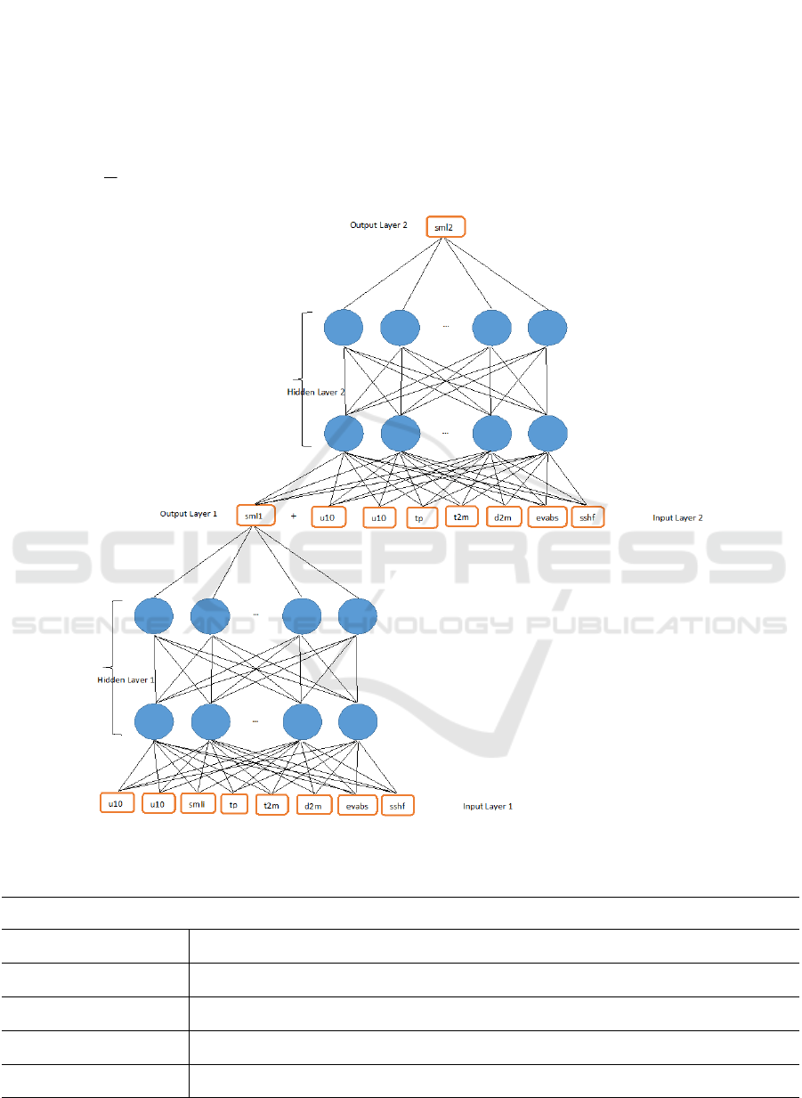
We opt to a two-hidden layer regression neural

network. The output of the previous layer is the input

of the next layer. It is a deep neural network

regression and its mathematical structure is composed

by:

- An input layer for which the number of nodes is

equal to the number of input parameters.

- Hidden layers node composed of neurons.

- The regression model output layer. The output of the

previous hidden layer is multiplied by the weight and

is added to a bias on the output node to obtain the

regression prediction value.

We use a single model to predict soil moisture for

layer 1 and layer 2, so-called 2NNL2. This model is a

succession of two networks to form a unique model.

The first network has as input the eight parameters

and as output the soil moisture of layer 1. The second

network have as input the same inputs of the previous

network plus the output of network 1. The output is

the soil moisture of layer 2.

We use five models to predict the soils moisture

level multiple days in advance.

Model 1: The output data of network 1 (sml1) is

measured two (02) days after the input data. The

output data of network 2 (sml2) is measured three (03)

days after the input data and one (01) day after the

sml1.

Model 2: The output data of network 1 (sml1) is

measured three (03) days after the input data. The

output data of network 2 (sml2) is measured four (04)

days after the input data and one (01) day after the

sml1.

Model 3: The output data of network 1 (sml1) is

measured four (04) days after the input data. The

output data of network 2 (sml2) is measured five (05)

days after the input data and one (01) day after the

sml1.

Model 4: The output data of network 1 (sml1) is

measured five (05) days after the input data. The

output data of network 2 (sml2) is measured six (06)

days after the input data and one (01) day after the

sml1.

Model 5: The output data of network 1 (sml1) is

measured six (06) days after the input data. The

output data of network 2 (sml2) is measured seven

(07) days after the input data and one (01) day after

the sml1.

This means that for each model, the inputs of network

2 are the same inputs of network 1 plus output of

network 1 (sml1).

After many attempts, all these models’ structure

was determined to be 8-150-80-1 followed by 8-100-

50-1 respectively for network 1 and network 2.

We train and optimize Model 1, Model 2, Model

3, Model 4 and Model 5.

Several algorithms can be used for optimization.

Here we choose Adaptive Gradient Algorithm

(AdaGrad) as an optimization algorithm (Duchi et al.,

2011). AdaGrad is an optimization algorithm for

gradient-based optimization. AdaGrad performs

gradient descent with a variable learning rate.

Parameters associated with infrequent features are

adapted with large gradients and parameters

associated with frequently occurring features perform

small gradients. Adagrad thus improves on SGD, or

stochastic gradient descent, with a per-node learning

rate scheduler built into the algorithm.

To optimize gradient descent at time-step t,

an objective function







is minimized by updating

a parameter



. The equation of the parameter is:

GdiagI









)(







(3)

where



is the parameter to be updated at time-step

t, η is the learning rate, ε is some small quantity that

used to avoid the division of zero, I is the identity

Soil Moisture Prediction Model from ERA5-Land Parameters using a Deep Neural Networks

391

matrix,

)(

Gdiag

is a diagonal matrix containing the

squares of all previous gradients,

is the vector of

gradients for the current time-step and can be

expressed, for each training example

and label

, by:





yxJ

),,(



(4)

The accuracy on the learning set is 93.8% and the

validation accuracy is 92.5% for all models. The

mean absolute error turn around 0.015 m

for

training phase and 0.02 m

for validation phase.

Table 1 summarizes performances measures for all

models. We notice that the soil moisture retrieved

from training features and its real values are quite

good for layer 1 and layer 2. This figure gives us an

idea of the accuracy of the model in reproducing the

training dataset.

Figure 1: A two connected two-hidden layer regression neural network (2NNL2).

Table 1: Performance measures of 2NNL2 models.

Train mae Test mae Train loss Test loss Train R

Test R

Model 1

Output 1 0.010 0.013 0.0002 0.0005 98.37% 98.43%

Output 2 0.023 0.026 0.0010 0.0013 93.8% 93.7%

Model 2

Output 1 0.013 0.015 0.0004 0.0006 97.7% 97.2%

Output 2 0.023 0.026 0.0011 0.0014 93.8% 92.7%

Model 3

Output 1 0.015 0.018 0.0005 0.0007 97.1% 97.1%

Output 2 0.023 0.027 0.0010 0.0015 93.8% 92.5%

Model 4

Output 1 0.017 0.020 0.0006 0.0009 96.8% 96.5%

Output 2 0.024 0.027 0.0011 0.0013 93.9% 92.7%

Model 5

Output 1 0.018 0.021 0.0006 0.0010 96.4% 96.4%

Output 2 0.024 0.027 0.0011 0.0014 93.6% 92.5%

NCTA 2020 - 12th International Conference on Neural Computation Theory and Applications

392

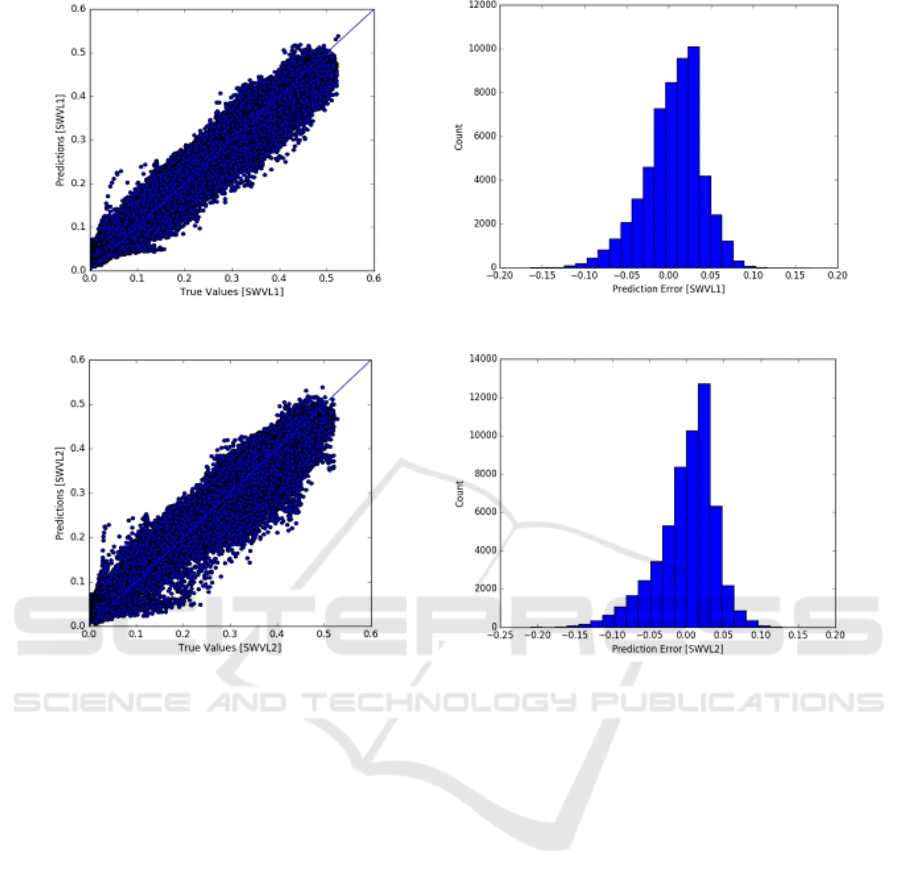
Figure 2: Scatter plot (left) and relative error (right) between predicted and measured values for sml1 in 12 July, 2012.

Figure 3: Scatter plot (left) and relative error (right) between predicted and measured values for sml2 in 13 July, 2012.

4 RESULTS

In the training phase, the dataset selected concern

sample less than 20% of all measured values from

July to December 2012. We compared two data sets

of soil moisture that did not participate in training

phase to the measure from ERA5-Land at the same

date.

Using July 10, 2012 input parameters, we predict

sml1 and sml2 two days and three days in the future,

respectively, i.e. on dates of 12 and 13 July, 2012.

Figure 2 and figure 3 show comparisons of soil

moisture layer predicted and measured. We can

notice that the prediction model was able to retrieve

the soil moisture very faithfully. The accuracies of

scatter diagrams are 95.6% and 94.4% respectively

for sml1 and sml2.

The global mean absolute error between the two

data sets is quite small: 0.03 m

. Then, the sml1

retrieval from the Era5-Land features by using neural

network are obtained with good accuracy. In the

construction of the model, the output sml1 of the first

stage is part of the input of the second stage which

models the sml2. This means that a good estimate of

the output of stage 1 will lead to a good estimate of

stage 2. The contrary will also cause the opposite

effect. These comparisons on dataset that not

participate to the training phase between observed

and estimated show the generalization capability of

the built model.

Soil moisture obtained from Climate Change

Initiative of the European Space Agency (CCI-ESA),

which are combination of measurements from various

single-sensor active and passive microwave, is used

to validate mainly our model and occasionally the

ERA5-Land data.

Comparison between the sml1 predicted two days

in the future from model with using the ERA5-Land

parameters reanalysis (a) and the measured ESA-CCI

sml1 (b) on July 10, 2012 can be seen in figure 4. The

soil moisture prediction two days in the future was

compared with measurements from ESA-CCI data. A

correlation of 87% and a mean absolute error of 0.05

were obtained. For the prediction made two

Soil Moisture Prediction Model from ERA5-Land Parameters using a Deep Neural Networks

393

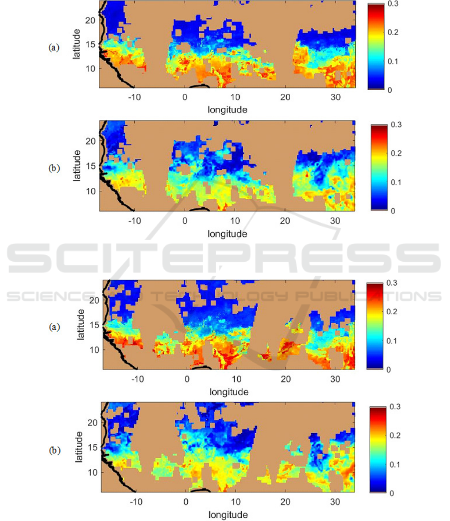
days in the future for layer 1 in figure 5 (date of July

12, 2012), we also note good results with a correlation

coefficient of 85% and a mean absolute error of 0.06

. For the two figures shown below, we note that

the trends are the same in part (a) and part (b).

However, the intensities of soil moisture predicted

from Era5-Land features are on average 0.05 m

-3

higher than those measured from CCI-ESA.

Figure 4: Map of the soil moisture layer 1 predicted from ERA5-Land features with 2NNL2 (a) and CCI-ESA observations

data (b) in 10 July, 2012.

Figure 5: Map of the soil moisture layer 1 predicted from ERA5-Land features with 2NNL2 (a) and CCI-ESA observations

data (b) in 12 July, 2012.

NCTA 2020 - 12th International Conference on Neural Computation Theory and Applications

394

5 CONCLUSIONS

In this study, dataset from ERA5-Land were used to

build a prediction model by using a deep neural

network able to evaluate further soil moisture in the

first two layers. The built model, so-called 2NNL2,

which is a succession of two-hidden layers, retrieved

successfully soil moisture layer 1 and layer 2 for two

to seven days in the future. We have analyzed the

performance of the model by comparing soil moisture

estimated from ERA5-Land features to CCI-ESA soil

moisture. We denoted that results are satisfying with

low mean absolute error and high correlation.

REFERENCES

Balsamo, G., Albergel, C., Beljaars, A., Boussetta, S., Brun,

E., Cloke, H., Dee, D., Dutra, E., Muñoz-Sabater, J.,

Pappenberger, F., de Rosnay, P., Stockdale, T., Vitart,

F., 2015. ERA-Interim/Land: a global land surface

reanalysis data set. Hydrol. Earth Syst. Sci. 19, 389–

407.

Cai Y., Zheng W., Zhang X., Zhangzhong L., Xue X.,

(2019) “Research on soil moisture prediction model

based on deep learning”. PLoS ONE 14(4): e0214508.

https://doi.org/10.1371/journal.pone.0214508

Chen XF, Wang ZM, Wang ZL, Li R. Drought evaluation

and forecast model based on soil moisture simulation.

China Rural Water and Hydropower, 2014(05): 165–

169.

Diouf D. and Seck D., (2019) “Modeling the chlorophyll-A

from sea surface reflectance in West Africa by deep

learning methods: A comparison of multiple

algorithms”. International Journal of Artificial

Intelligence & Applications; 2019; Vol 10(6); Pages

33-40

Kaleita A. L., Tian L. and Yao H., “Soil moisture estimation

from remotely sensed data,” in American Society of

Agricultural Engineers Annual International meeting,

Las Vegas, NV, July 27-30, 2003.

Duchi, J., Hazan, E., & Singer, Y. (2011). Adaptive

Subgradient Methods for Online Learning and

Stochastic Optimization. Journal of Machine Learning

Research, 12, 2121–2159.

LeCun Y. A., Bottou L., Orr G. B., and Müller K.-R.,

“Efficient backprop,” in Neural Networks: Tricks of the

Trade, pp. 9–48, Springer, Berlin, Germany, 2012.

Miralles, D.G., Teuling, A.J., van Heerwaarden, C.C., Vila-

Guerau de Arellano, J., 2014. Mega-heatwave

temperatures due to combined soil desiccation and

atmospheric heat accumulation. Nat. Geosci. 7, 345–

349.

Mueller, B., Seneviratne, S.I., 2012. Hot days induced by

precipitation deficits at the global scale. Proc. Natl.

Acad. Sci. 109 (31), 12398–12403.

Philippon N. et Fontaine B., 2002: The relationship

between the Sahelian and previous 2nd Guinean rainy

seasons: a monsoon regulation by soil wetness?

Annales Geophysicae, 20(4), 575-582.

Schlesinger W H, Jasechko S. Transpiration in the global

water cycle. Agricultural and Forest Meteorology,

2014, 189: 115–117.

Seneviratne, S.I., Corti, T., Davin, E.L., Hirschi, M., Jaeger,

E.B., Lehner, I., Orlowsky, B., Teuling, A.J., 2010.

Investigating soil moisture-climate interactions in a

changing climate: a review. Earth Sci. Rev. 99, 125–

161.

Sultan B. et Janicot S., 2000: Abrupt shift of the ITCZ over

West Africa and intra- seasonal variability. Geoph. Res.

Lett., 27, 3353-3356.

Vahedberdi S., Saskia V. and Stroosnijder L. “A simple

model to predict soil moisture: Bridging Event and

Continuous Hydrological (BEACH) modelling”,

Environmental Modelling & Software Volume 24,

Issue 4, April 2009, Pages 542-556

Veres M, Lacey G, Taylor G W. Deep learning

architectures for soil property prediction. Computer and

Robot Vision (CRV), 2015 12th Conference on. IEEE,

2015: 8–15.

Soil Moisture Prediction Model from ERA5-Land Parameters using a Deep Neural Networks

395