
Improving the Transparency of Deep Neural Networks using Artificial
Epigenetic Molecules
George Lacey
1 a
, Annika Schoene
1 b
, Nina Dethlefs
1 c
and Alexander Turner
2 d
1
Department of Computer Science, University of Hull, Cottingham Rd, Hull HU6 7RX, U.K.
2
Department of Computer Science, University of Nottingham, Wollaton Rd, Lenton, Nottingham NG8 1BB, U.K.
Keywords:
Deep Learning, XAI, Transparency, Epigenetics, Gene Regulation Models.
Abstract:
Artificial gene regulatory networks (AGRNs) are connectionist architectures inspired by biological gene reg-
ulation capable of solving tasks within complex dynamical systems. The implementation of an operational
layer inspired by epigenetic mechanisms has been shown to improve the performance of AGRNs, and improve
their transparency by providing a degree of explainability. In this paper, we apply artificial epigenetic layers
(AELs) to two trained deep neural networks (DNNs) in order to gain an understanding of their internal work-
ings, by determining which parts of the network are required at a particular point in time, and which nodes
are not used at all. The AEL consists of artificial epigenetic molecules (AEMs) that dynamically interact with
nodes within the DNNs to allow for the selective deactivation of parts of the network.
1 INTRODUCTION
Deep neural networks (DNNs) are an implementa-
tion of machine learning that are capable of automatic
feature detection. Their abstract nature means that
they are applicable to many domains such as speech
recognition and face detection (Ding and Tao, 2015;
Nassif et al., 2019; Lifkooee et al., 2019; Zhang
et al., 2019); however, this comes at the cost of trans-
parency. The ‘black-box’ nature of deep neural net-
works means that it is difficult to determine why a
neural network is making the decisions that result in
its output, which is problematic for a multitude of
reasons. Neural networks have no understanding of
the context behind data, so decisions may be made
based on trends within the training data that do not
fit with existing theory of the subject. For exam-
ple, a neural network deployed on pneumonia patients
determined that patients with asthma had a low risk
of dying, when in reality this does not make sense
(Caruana et al., 2015; Adadi and Berrada, 2018). In
this case, it would have been useful for a healthcare
professional to know the reason behind this decision,
so that they could recognise the fault in the system.
a
https://orcid.org/0000-0003-0494-2460
b
https://orcid.org/0000-0002-9248-617X
c
https://orcid.org/0000-0002-6917-5066
d
https://orcid.org/0000-0002-2392-6549
Moreover, in (Nguyen et al., 2015) it was shown that
very accurate convolutional neural networks are eas-
ily fooled, often classifying images with high accu-
racy which bear no resemblance to the classification
the network prescribed. This reasoning also applies
at the point of designing the neural network, when
trying to improve the accuracy of neural networks it
would be useful to see which conditions are causing
issues. The field of explainable AI (XAI) attempts to
address the black-box nature of neural networks with
the development of techniques to expose the internal
mechanics of them (Cortez and Embrechts, 2013; Che
et al., 2015; Hailesilassie, 2016; Oh et al., 2019).
Genes are segments of DNA used to create
gene products such as proteins, essential complex
molecules that are involved in many of the biochem-
ical reactions that occur to keep an organism alive.
Gene regulation is the mechanism that controls the
transcription of genes, which is necessary in order to
produce the different functionality across cell types
within an organism, and to prevent wasted energy
from the unnecessary synthesis of gene products. Ro-
bustness is an important quality of gene regulatory
networks, so that functionality persists despite inter-
nal and external perturbations (Kitano, 2004; Mac-
Neil and Walhout, 2011). They are also adaptive
to changes in the organism’s environment (Gracey,
2007; Hoffmann and Willi, 2008), so that a popula-
tion survives changing conditions. These characteris-
Lacey, G., Schoene, A., Dethlefs, N. and Turner, A.
Improving the Transparency of Deep Neural Networks using Artificial Epigenetic Molecules.
DOI: 10.5220/0010105301670175
In Proceedings of the 12th International Joint Conference on Computational Intelligence (IJCCI 2020), pages 167-175
ISBN: 978-989-758-475-6
Copyright
c
2020 by SCITEPRESS – Science and Technology Publications, Lda. All rights reserved
167

tics prompted computational models to be produced
such as the ‘Artificial Genetic Network’ (AGRN), ca-
pable of solving tasks in chaotic environments despite
its simple, abstract nature (Lones et al., 2010). The
addition of a layer inspired by epigenetics has been
found to improve the performance, transparency, and
even allow for a degree of manual control over the
networks (Turner et al., 2013; Turner and Dethlefs,
2017).
In this paper, we apply an epigenetic layer consist-
ing of artificial epigenetic molecules to two DNNs,
connectionist architectures not inspired by the inter-
actions of gene regulation in an attempt to determine
if the transparent properties of previous epigenetically
inspired architectures can be applied to DNNs. The
content of the paper is arranged as follows: the back-
ground of gene regulation and how this has inspired
computational analogues will be described, followed
by a description of the model used, the experimental
methodology will then be detailed, and finally a con-
clusion will be made.
2 BIOLOGICAL GENE
REGULATION
Proteins are complex molecules that perform a variety
of functions within biological organisms (Henzler-
Wildman and Kern, 2007), examples include en-
zymes, which act as catalysts during biochemical re-
actions, and messenger proteins, which coordinate
processes involving different types of tissues and or-
gans. Proteins are a gene product, a result of gene
expression where genes are transcribed from DNA to
produce RNA, which is translated into a polypeptide
sequence. The polypeptide sequence, sometimes in
conjunction with other polypeptide sequences forms
the final gene product. Higher order multicellular
organisms are composed of many different tissues
which are made up of different cell types such as mus-
cle and skin cells, each with their own properties. The
function of a cell is determined by the proteins that
are produced by the DNA within the cell. Gene regu-
lation is the process that determines which genes will
be transcribed from the cell’s DNA.
2.1 Epigenetics
The term ‘epigenetics’ has developed since its incep-
tion, as it was originally used to refer to epigene-
sis (Haig, 2004), a theory now generally accepted.
The term was also used to refer to all of the inter-
actions that occur between genes and their external
environment to result in phenotypic changes to an or-
ganism (Waddington et al., 1939; M
¨
uller and Olsson,
2003). A modern use of the term derived from this
is “the study of mitotically and/or meiotically herita-
ble changes in gene function that cannot be explained
by changes in DNA sequence” (Riggs et al., 1996),
this is the definition to which we will adhere in this
paper. This definition specifies that changes are heri-
table, meaning that they are passed down to an organ-
ism’s offspring. It also specifies that the changes are
caused by changes to the DNA nucleotide sequence.
In complex eukaryotic organisms, DNA must be
condensed into chromatin so that it may fit within the
nucleus of the organism’s cells. Chromatin is formed
by chains of nucleosomes formed as approximately
146 base pairs of DNA coiled around a histone oc-
tamer (a group of histone proteins). Chromatin acts as
an indexing system, providing RNA polymerase and
transcription factors access to the underlying DNA so
that transcription can occur (Phillips and Shaw, 2008).
The DNA in chromatin is generally inaccessible to the
transcriptional machinery. Chromatin remodelers are
complexes consisting of multiple proteins that alter
the structure of nucleosomes to allow for processes
such as transcription (Murawska and Brehm, 2011),
DNA repair (Chai et al., 2005) and chromatin assem-
bly (Polo and Almouzni, 2006).
3 GENE REGULATION MODELS
Artificial gene regulatory networks (AGRNs) are
models of gene regulation that are usually designed
to serve one of two purposes. Models may be created
by geneticists to simulate the dynamics of biological
gene regulation in order to improve the understanding
of it (Keedwell et al., 2002; Kauffman et al., 2003).
Models may also be created to capture the useful
properties found within gene regulation to apply
them to computational problems (White et al., 2005;
Lones et al., 2010). In this work, we will attempt
to use a model inspired by epigenetics to act on a
connectionist architecture in order to improve our
understanding of it. Robustness to internal and
external perturbations and adaptability are properties
found within biological gene regulation, and have
been shown to be present in computational models
(Turner et al., 2013; Turner et al., 2017).
More formally, this AGRN architecture can be de-
fined by the tuple hG, L, In, Outi, where:
G is a set of genes {g
0
. . . g
|G|
: g
i
= ha
i
, I
i
, W
i
i}
where:
a
i
: R is the activation level of the gene.
ECTA 2020 - 12th International Conference on Evolutionary Computation Theory and Applications
168

I
i
⊆ G is the set of inputs used by the gene.
W
i
is a set of weights, where 0 ≤ w
i
≤ 1,
|W
i
| = |I
i
|.
L is a set of initial activation levels, where |L
N
| = |N|.
In ⊂ G is the set of genes used as external inputs.
Out ⊂ G is the set of genes used as external outputs.
The ‘Random Boolean Network (RBN)’ was an
attempt to model interactions between genes by mod-
elling them as binary functions. The behaviour of
the network is a function of the interactions between
genes. Despite their simplicity, RBNs have been
shown to exhibit short and stable cycles, and be-
have with similarity to biological gene regulatory net-
works (Kauffman et al., 2003). The artificial genetic
network (AGRN) (Lones et al., 2010) brought the
RBN model into continuous space, and allowed for
the control of an external chaotic dynamical system.
Variables from the external system’s environment are
mapped onto the expression levels of genes within the
AGRN. The AGRN is then executed over a number of
time steps by calculating the expression levels of the
genes within the network. An output can be derived
from the network in the form of a set of expression
levels from allocated genes, used to control the exter-
nal system.
Epigenetic frames are a basic implementation of
an epigenetic layer that act on a continuous AGRN,
inspired by chromatin modifications and DNA methy-
lation. During the evolution of the AGRN, genes
may be allocated to different objectives. This al-
lowed genes to be switched off when they were not
needed, and improved the performance of the net-
works (Turner et al., 2012). This design was devel-
oped into epigenetic molecules, that interact directly
with the genes in the network and disable the genes
they are connected to if the molecule is active. The
advantage over this method was that the epigenetic
molecules automatically allocated genes to the objec-
tive that they were used to solve (Turner et al., 2013).
The epigenetic layer in this paper implements epige-
netic molecules that operate in a similar way; how-
ever, they are evolved separately to the training of the
connectionist architecture they are operating on.
4 THE ARTIFICIAL EPIGENETIC
MOLECULE
The artificial epigenetic molecule (AEM) is a unit that
takes in a given number of inputs, and processes them
using a regulatory function to determine whether it
is active. If active, the molecule will bring about a
0.42
0.62
0.16
0.14
0.63
0
0.62
0
0.14
0.63
Figure 1: Example of epigenetic molecule connectivity in
a connectionist architecture. Regular nodes are represented
by red circles, and epigenetic molecules in blue. Each node
within the network has an output, indicated by the number.
If the expression level of an epigenetic molecule is greater
than 0.5, it is active and disables the nodes it is connected to
by setting their expression levels to 0. The left graph shows
the network before the activated epigenetic molecule has
disabled the nodes that it is connected to, the right graph
shows the effects of the activated molecule, disabling two
nodes.
change to its outputs. In the case of AGRNs, the
inputs and outputs of the epigenetic molecules were
nodes within the network; however, in this work they
have been abstracted to function within other con-
nectionist architectures. An epigenetic molecule acts
similarly to a chromatin remodeler, in that it forms
connections with the external connectionist architec-
ture and selectively switches parts of it on or off, as a
chromatin remodeler provides selective access to the
underlying DNA.
An AEM operates by taking a sum of its inputs
(Equation. 2), and processing them using its regu-
latory function (Equation. 1) to produce its output.
This differs slightly to other models of gene regula-
tory networks as the connections are not weighted,
this is due to the fact that the connectionist archi-
tecture is responsible for its own weighting, and for
computational simplicity, so that analysis is easier.
A parametrised sigmoid function (Fig. 2) is used as
the regulatory function of the epigenetic molecules.
The weighted sum of the molecule inputs is used as
the input to the sigmoid function. Two parameters
control the properties of the sigmoid function. The
slope parameter s controls the steepness of the sig-
moid, higher values causing it to act more similarly
to a step function. The offset parameter b allows the
sigmoid to be repositioned along the x-axis. The pa-
rameters of the sigmoid function allow for different
behaviour that is determined during the evolution of
epigenetic molecules.
f (x) = (1 +e
−sx−b
)
−1
(1)
x =
n
∑
j=1
i
j
(2)
Improving the Transparency of Deep Neural Networks using Artificial Epigenetic Molecules
169
−5
0
5
0.5
1
x
σ(x)
Figure 2: The sigmoid function acts as the regulatory func-
tion within an AEM, to process its inputs. The slope and
offset parameters allow for more diverse behaviour.
Within this work, multiple AEMs are deployed to
act on neural networks over two separate data sets
to understand their functionality over different prob-
lems. The AEMs will act between the two hidden
layers of the networks. The output of several nodes
from the first hidden layer will act as the inputs to the
AEM. The nodes from the second hidden layer will
be controlled by the AEM, and will be ‘switched off’
if an AEM connecting to them is activated. The max-
imum number of inputs and outputs of the AEMs will
be limited. AEMs have been designed to dynamically
interact with the neural networks, meaning that they
are capable of changing their behaviour based on the
state of the network at any given epoch. This is advan-
tageous over traditional pruning techniques as parts of
the networks can be selectively controlled based not
only on the input data, but also how the networks in-
terpret and extract features from the input data. They
have been designed with simplicity in mind, adher-
ing to two principles. The first, is that their connec-
tivity is absolute; it is possible to determine exactly
which ANN nodes they are connected to. The sec-
ond, is that they have only two states—they are either
active or inactive. There is potential for AEMs to ex-
hibit more complex behaviour; for example, the con-
nections to nodes could be weighted. Unfortunately,
this would increase the difficulty of analysing the net-
works, potentially resulting in the extra task of inter-
preting AEMs, which could be considered paradox-
ical as we are trying to improve the transparency of
connectionist architectures. The AEL can be consid-
ered as a collection of AEMs.
5 EXPERIMENTATION
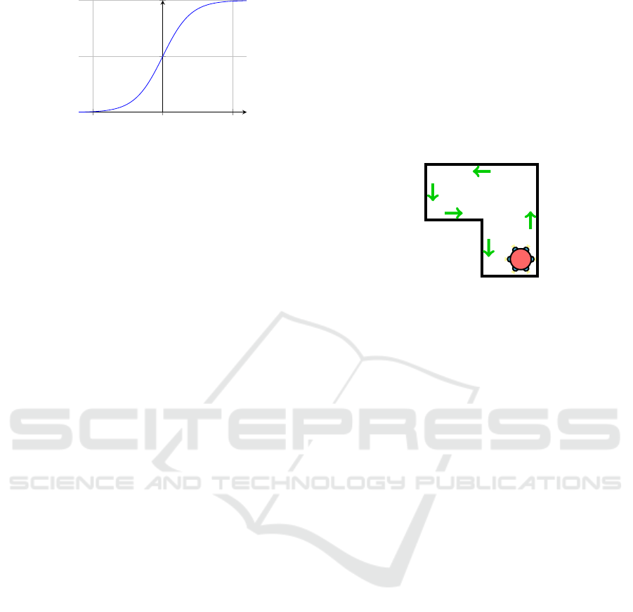
5.1 Wall following Robot Dataset
The first neural network was trained on a dataset col-
lected as a robot navigated a room by following the
wall of the room in an anti-clockwise direction (Freire
et al., ) (shown by Figure. 3). 24 sensors arranged
around the circumference of the robot collected ul-
trasound readings at a rate of 9 per second, consti-
tuting the attributes of the dataset. Sensor readings
were collected a total of 5456 times. The class la-
bel of the dataset is the movement of the robot in
that time step, recorded as moving forward, turning
slightly left, turning slightly right, or turning sharply
right.
Figure 3: Top-Down illustration of a wall following robot
traversing a room similarly to the robot that collected the
ultrasound data. This robot has only 6 ultrasound sensors,
as indicated by the blue circles. The green arrows show the
path that the robot will take.
5.2 Cardiotocography Dataset
Cardiotocography (CTG) is a method of recording
the fetal heartbeat and uterine contractions during
pregnancy used to monitor the well-being of the foe-
tus. The second dataset we will use consists of fea-
tures generated from 2126 cardiotocography readings
(Marques et al., ). The neural network will be trained
to predict the fetal state, consisting of labels normal,
suspect, and pathologic. A foetus classed as normal
suggests that the foetus is healthy and no action needs
to be taken. A foetus classed as suspect indicates that
that some readings are abnormal and action may need
to be taken in order to ensure the health of the foetus,
and that further monitoring should take place. A foe-
tus classed as pathologic indicates that multiple prob-
lems have been found in the readings, and that im-
mediate action needs to be taken to correct reversible
causes of the abnormal readings. Records with miss-
ing values will be removed from the dataset before
training the neural network.
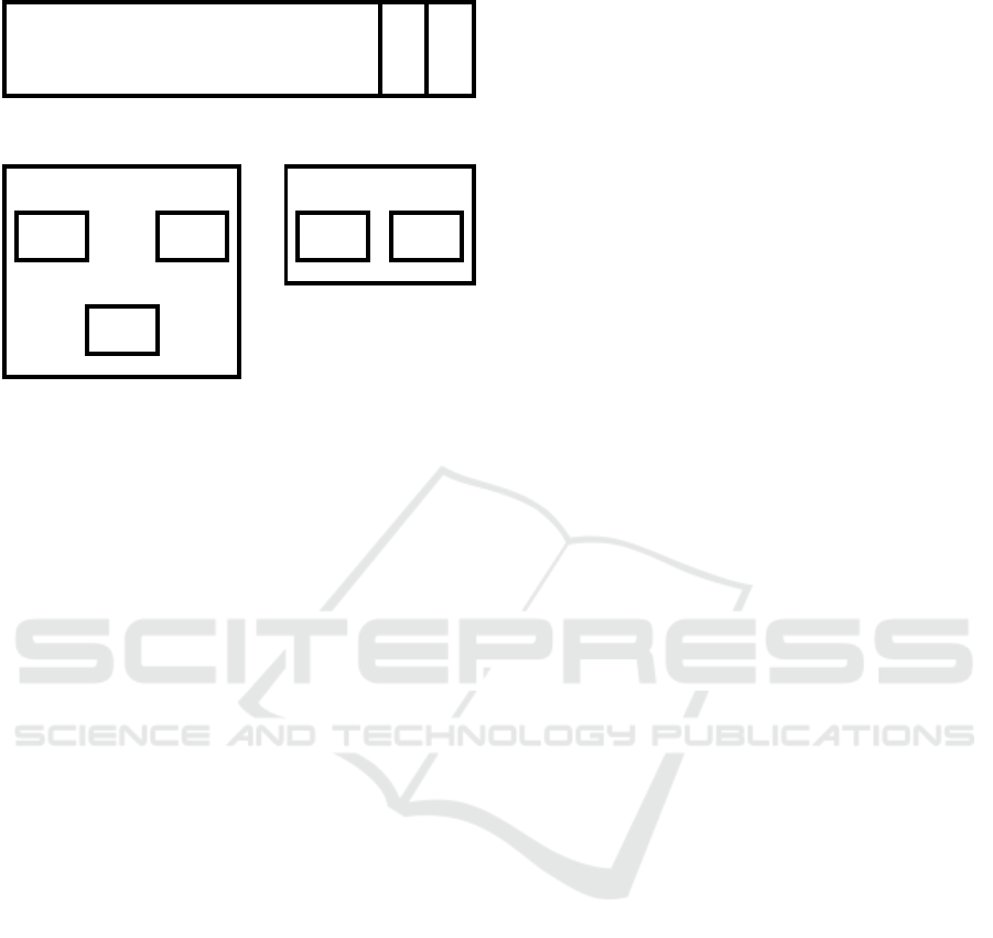
The datasets were split into three subsets (Fig-
ure. 4). Subsets A, B and C were used as the train-
ing, validation, and test set respectively when training
the neural network. Set B was used as the training
set when evolving the epigenetic layer, and set C was
used to evaluate their effects on the performance of
the neural network. Set C is never seen during the
training phase of the ANN or the AEL, so that the per-
formance of both can be evaluated with unseen data.
ECTA 2020 - 12th International Conference on Evolutionary Computation Theory and Applications
170
Dataset
A B C
ANN training
Training
A
Test
C
Validation
B
AEL Training
Evolution
B
Test
C
Figure 4: This diagram shows how the wall following robot
dataset was split into subsets, and how the subsets were used
to train the artificial neural network (ANN) and the artificial
epigenetic layers (AEL). Note that set C is never seen dur-
ing the training of the ANN, or the evolution of the AELs.
5.3 Neural Network
Neural networks consisting of two hidden layers will
be trained on the datasets produced by the wall fol-
lowing robot and the cardiotocography machine. The
first hidden layer contains 16 nodes, and the second
24. Both hidden layers use the ReLU activation func-
tion and are trained with dropout, the output layer
uses the softmax activation function. The first hid-
den layer has a dropout of 20%, and the second 10%.
Training was halted when the evaluation performance
against the validation set started to decrease, to reduce
the chance of overfitting the training data.
The abstract and black-box nature of neural net-
works means that it is difficult to construct them with
an optimal architecture without resorting to trial and
error. This has prompted the use of heuristics such
as evolutionary algorithms (Shrestha and Mahmood,
2019; Lu et al., 2019) to find an optimal architecture.
Techniques have been developed to act on neural net-
works that have already been trained; pruning neural
networks is the act of removing redundant weights to
reduce the overall size of the network. This is bene-
ficial as it has the potential to reduce the computation
time and space in memory when running such net-
works (LeCun et al., 1990; Han et al., 2015b; Han
et al., 2015a), allowing them to run on cheaper and
simpler architectures. We will attempt to discover re-
dundant nodes within the neural networks in this pa-
per using the artificial epigenetic layer.
5.4 Artificial Epigenetic Layer
An external artificial epigenetic layer has been con-
structed to act on top of the trained neural net-
works. The layer consists of 16 epigenetic molecules,
this number has been chosen as it is the number of
nodes in the second hidden layer of the neural net-
works, meaning that it is possible for each node to
be switched independently, but does not necessarily
mean that each epigenetic molecule will control a dif-
ferent node. The number of input and output nodes
that the AEMs may connect to has been limited so
that individual molecules perform smaller actions that
are easier to analyse. The number of outputs an AEM
may connect to is limited to 1, so that a given AEM
may be easily associated with a single neural network
node, and the number of inputs limited to 3.
The epigenetic layer is evolved using a genetic
algorithm (GA) with a population size of 512. The
maximum number of generations has been set to 300;
however, early termination will occur if no improve-
ment in performance has been found after 10 gener-
ations. The population consists of members, where
each member is a set of AEMs, each with a set of in-
puts and outputs. In terms of encoding, each member
consists of a set of values representing the parame-
ters of the activation function and the inputs and out-
puts it is connected to, they are constrained so that
they may only be set to valid values during the ex-
ecution of the GA. Members are evaluated via their
fitness function, which is used to sort them based on
how successful they are at solving the task. In this
case, the fitness function returns 0 if the epigenetic
layer causes the neural network performance to de-
crease upon application, as it is not desirable for the
epigenetic molecules to have a negative impact on the
network. If the epigenetic layer does not decrease
the performance of the neural network, it returns the
average percentage of weights zeroed in the network
over time. Each time the population advances, a set
of 8 ‘elite’ members will be copied directly to the
new generation, these are the top performing mem-
bers, and are retained so that they are not lost due to
random chance.
Two genetic operators are applied to the popula-
tion at each generation. The recombination operator
combines 2 members of the population (the parents)
to produce 2 new members (the offspring). The par-
ents are combined by swapping over attributes, in this
case, the inputs and outputs of each AEM. The inten-
tion of applying the mutation operator is to produce
offspring that contain desirable traits from two par-
ents that have unique desirable traits. To increase the
chance of parents with desirable characteristics being
Improving the Transparency of Deep Neural Networks using Artificial Epigenetic Molecules
171

chosen, they are selected using the tournament selec-
tion algorithm. An ‘arena’ of 16 random members
is created, and the member with the highest fitness
function is chosen. Parents have a 50% chance of re-
combining, if they are not recombined, they will be
copied directly to the next generation. The mutation
operator iterates through the attributes of each mem-
ber and has a 20% chance of randomly changing it
to another valid value. The intention of applying the
mutation operator is to introduce new characteristics
to the population, it has been set to occur to approxi-
mately 20% of the attributes as a compromise. If the
mutation probability is too low, new characteristics
will not be introduced quickly enough and the popu-
lation will develop slowly; if mutation occurs too of-
ten, desirable traits are more likely to be lost and the
process occurs similarly to a random search.
Algorithm 1: Execute genetic algorithm.
1: P ← {} {Initialise initial empty population}
2: for x = 1 → Population size do
3: P ← P ∪ Randomly initialised AGRN
4: end for
5: for y = 1 → Number of generations do
6: for all p ∈ P do
7: EVALUATE(p)
8: end for
9: Q ← {} {Initialise empty child population}
10: Q ← Q ∪ ELITE MEMBERS
11: repeat
12: R ← TOURNAMENT SELECT(P)
13: R ← R ∪ TOURNAMENT SELECT(P)
14: if RANDOM CHANCE then
15: RECOMBINE(R)
16: end if
17: Q ← Q ∪ R
18: until |Q| is Population size
19: P ← Q
20: MUTATE(P)
21: end for
6 RESULTS
Five individually evolved artificial epigenetic layers
(AELs) were optimised to act on each of the neu-
ral networks separately. Each of the 5 AELs acts
as a repeat experiment, so that their behaviours can
be compared. The AELs are restricted to connected
to 3 nodes from the first hidden layer of the neural
None
1 2 3 4 5
80
85
90
95
100
92.86
87.18
86.08
86.26
86.08
85.9
Epigenetic Layer
% Performance
Figure 5: This bar graph shows how the application of each
of the epigenetic layers impacted the performance of the
wall following robot neural network. There is an approx-
imate 5-7% decrease in performance when the masks are
applied. The performance of the neural network without an
AEL applied is shown by the ‘None’ column. Note that the
lower bound of the y axis is 80%.
networks, and a single node from the second hidden
layer. During training, the fitness of the AELs was set
to zero if they had a negative impact on the perfor-
mance of the neural networks, as it is undesirable to
reduce the performance of the networks in the pro-
cess of improving its transparency. When evaluat-
ing the performance of the neural networks with the
AELs applied on the test set, the performance of them
decreased slightly, as shown by Figure. 5 and Fig-
ure. 6. This is to be expected, as the subset of data
used to evolve the AEL contained only 10% of the
dataset. The performance of the ANN did not drop
below 85%, so the effects were not catastrophic.
6.1 Purged Nodes
If an epigenetic molecule is active 100% of the time,
it has effectively removed its output node from the
ANN. We will refer to a node in this state as being
‘purged’, and it is likely that the node is not needed
in the network. Table. 1 displays which nodes from
the second layer of the ANNs have been purged by
each AEL. The number of nodes purged in both net-
works is surprisingly high, which indicates the poten-
tial for reducing the size of the networks. The oc-
currence of each node purged in the network predict-
None
1 2 3 4 5
80
85
90
95
100
95.77
94.84
92.49
93.9
92.96
95.31
Epigenetic Layer
% Performance
Figure 6: This bar graph shows how the application of each
of the epigenetic layers impacted the performance of the
cardiotocography neural network. There is an approximate
0.5-2% decrease in performance when the masks are ap-
plied. The performance of the neural network without an
AEL applied is shown by the ‘None’ column. Note that the
lower bound of the y axis is 80%.
ECTA 2020 - 12th International Conference on Evolutionary Computation Theory and Applications
172

ing the wall following robot dataset has been sum-
marised in Figure. 7. Node 14 is of interest as it is
purged in all the AELs, indicating that it is not cru-
cial. Similarly, nodes 5 and 11 are present in 4 out of
the 5 AELs, indicating that they may not be crucial to
the overall functionality of the ANN. Many nodes are
purged by a lesser amount of AELs, this may be due
to the fact that the AELs were not evolved through
enough generations. It could also indicate that dif-
ferent AELs have disabled different redundant parts
of the network. The occurrence of each node purged
in the network predicting the CTG dataset has been
summarised in Figure. 8. Nodes 10 and 13 have been
purged in 4 out of the 5 cases, strongly indicating that
they are not crucial for the ANN to function. Nodes 0,
1, 2, 5, 6 and 14 are purged in 2 out of the 5 networks,
the rest of the nodes featured in the graph were purged
inconsistently, which again could indicate that they
work in conjunction with other nodes, or that there
are redundancies within the network.
Table 1: Nodes purged by each epigenetic layer. Results
from the wall following robot dataset are shown in the left
table, and CTG in the right.
Layer Purged nodes
1 4, 5, 6, 9, 11, 13, 14
2 4, 5, 8, 9, 11, 14
3 7, 8, 11, 12, 13, 14, 15
4 5, 6, 10, 14, 15
5 3, 5, 8, 10, 11, 14, 15
Layer Purged nodes
1 1, 10, 13, 14, 15
2 2, 6
3 1, 8, 9, 10, 11, 13
4 0, 5, 10, 13, 14
5 0, 2, 5, 6, 10, 13
3 4 5 6
7
8 9 10 11 12 13 14 15
0
2
4
6
1
2
4
2
1
3
2 2
4
1
2
5
3
Node in second hidden layer
Count
Figure 7: This bar graph shows the amount of times a wall
following robot DNN node from the second hidden layer
has been purged by an AEL. The occurrence of a node is
likely to indicate its importance in the network.
6.2 Nodes Active based on Neural
Network Prediction
The dynamic behaviour of AEMs allow for nodes to
be selectively deactivated. We can utilise this be-
haviour to determine which parts of the DNN are
functionally relevant based on the prediction the net-
work has made. To demonstrate this, we will analyse
the first AEL acting on the wall following robot task,
and the fifth AEL acting on the CTG data.
0 1 2 5 6 8 9 10 11 13 14 15
0
2
4
2 2 2 2 2
1 1
4
1
4
2
1
Node in second hidden layer
Count
Figure 8: This bar graph shows the amount of times a Car-
diotocography DNN node from the second hidden layer has
been purged by an AEL. The occurrence of a node is likely
to indicate its importance in the network.
The activity of each node in the wall following
robot DNN that was selectively switched by an AEM
according to the network prediction has been sum-
marised in Table. 2. AEMs that are always active or
inactive, in addition to AEMs that do not have out-
puts have not been included as they do not show dy-
namic behaviour. The behaviour of the AEM control-
ling node 15 is of particular interest, as it is disabling
the node for a majority of the time that the ANN is
predicting a slight right turn, indicating that node 15 is
unlikely to be involved in the ANN’s decision to pre-
dict that class. Lower numbers indicate that a node is
likely to be required for the network to predict a par-
ticular task. All three nodes are never disabled when
the network is predicting a slight left turn, indicating
that they are likely to be required for the ANN to pre-
dict this.
The activity of each node in the CTG DNN that
was selectively switched by the fifth AEL based on
the network prediction has been displayed in Table. 3.
All three nodes are active approximately 50% of the
time when the network is predicting a normal state,
indicating that they are probably involved in predict-
ing this class. Nodes 1 and 15 are deactivated most
of the time when the network is predicting a suspect
case, indicating that they are not very involved in the
prediction of this class. All three nodes are very inac-
tive when the network is predicting a pathologic state,
indicating that they are not very involved when pre-
dicting this class.
Table 2: Nodes deactivated based on wall following robot
network prediction.
Node Time inactive
forward sh right sl left sl right
2 48.3% 18.8% 0% 29.3%
10 0.4% 29.3% 0% 51.2%
15 12.8% 8.2% 0% 92.7%
Improving the Transparency of Deep Neural Networks using Artificial Epigenetic Molecules
173

Table 3: Nodes deactivated based on CTG network predic-
tion.
Node Time inactive
normal suspect pathologic
1 53.0% 91.2% 15.4%
14 54.8% 35.3% 0%
15 53.0% 70.6% 7.7%
7 CONCLUSION
In this paper we have designed an artificial epige-
netic layer (AEL) to act externally on two deep learn-
ing networks (DNNs) in order to improve the trans-
parency of them. The AEL is constructed of artificial
epigenetic molecules (AEMs), designed with simplic-
ity in mind for ease of analysis. We will now conclude
with what our AEL has allowed us to achieve in the
scope of improving the transparency of the DNN, fol-
lowed by areas for improvement and further research.
Purging nodes is the process of effectively remov-
ing them from the network. The AEL has been shown
to be capable of purging nodes from the second layer
of the neural networks. This provides a basic level of
transparency as to which nodes are not crucial to the
functionality of the ANN. Purging nodes is also ben-
eficial as it reduces the overall size of the networks,
potentially reducing the processing time and space in
memory, which could allow for the networks to run
on simpler, cheaper architectures.
The activity of nodes was analysed based on the
prediction the networks were making at the time. This
primarily indicated which nodes within the networks
were required, for the networks to make such predic-
tions. Analysing the activity of nodes in this way
could help to describe the processing that is occur-
ring within the networks to determine the reasoning
behind the decisions that they are making.
The neural networks used during experimentation
solved relatively simple tasks, when considering other
tasks that DNNs excel at such as image recognition.
Future work may involve the application of AELs
to more complicated DNNs, which may help to un-
cover more complex network behaviour that would
further demonstrate the potential of AELs. To make
this more computationally feasible, a more efficient
AEL must be developed that interacts directly within
the implementation of the network. The subsets of
training data used to train the AELs was limited in
size due to the majority of the data being used to train
the ANN, training the AELs with more data is likely
to cause less of an ANN performance drop.
ACKNOWLEDGEMENTS
This work was supported by the Engineering and
Physical Sciences Research Council through the
Project entitled Artificial Biochemical Networks:
Computational Models and Architectures under Grant
EP/F060041/1
REFERENCES
Adadi, A. and Berrada, M. (2018). Peeking inside the black-
box: A survey on explainable artificial intelligence
(xai). IEEE Access, 6:52138–52160.
Caruana, R., Lou, Y., Gehrke, J., Koch, P., Sturm, M., and
Elhadad, N. (2015). Intelligible models for healthcare:
Predicting pneumonia risk and hospital 30-day read-
mission. In Proceedings of the 21th ACM SIGKDD
international conference on knowledge discovery and
data mining, pages 1721–1730.
Chai, B., Huang, J., Cairns, B. R., and Laurent, B. C.
(2005). Distinct roles for the rsc and swi/snf atp-
dependent chromatin remodelers in dna double-strand
break repair. Genes & development, 19(14):1656–
1661.
Che, Z., Purushotham, S., Khemani, R., and Liu, Y.
(2015). Distilling knowledge from deep networks
with applications to healthcare domain. arXiv preprint
arXiv:1512.03542.
Cortez, P. and Embrechts, M. J. (2013). Using sensi-
tivity analysis and visualization techniques to open
black box data mining models. Information Sciences,
225:1–17.
Ding, C. and Tao, D. (2015). Robust face recognition via
multimodal deep face representation. IEEE Transac-
tions on Multimedia, 17(11):2049–2058.
Freire, A., Veloso, M., and Barreto, G. Wall-
following robot navigation data set.
https://archive.ics.uci.edu/ml/datasets/Wall-
Following+Robot+Navigation+Data.
Gracey, A. Y. (2007). Interpreting physiological responses
to environmental change through gene expression pro-
filing. Journal of Experimental Biology, 210(9):1584–
1592.
Haig, D. (2004). The (dual) origin of epigenetics. In
Cold Spring Harbor Symposia on Quantitative Biol-
ogy, volume 69, pages 67–70. Cold Spring Harbor
Laboratory Press.
Hailesilassie, T. (2016). Rule extraction algorithm for
deep neural networks: A review. arXiv preprint
arXiv:1610.05267.
Han, S., Mao, H., and Dally, W. J. (2015a). Deep compres-
sion: Compressing deep neural networks with prun-
ing, trained quantization and huffman coding. arXiv
preprint arXiv:1510.00149.
Han, S., Pool, J., Tran, J., and Dally, W. (2015b). Learning
both weights and connections for efficient neural net-
work. In Advances in neural information processing
systems, pages 1135–1143.
ECTA 2020 - 12th International Conference on Evolutionary Computation Theory and Applications
174

Henzler-Wildman, K. and Kern, D. (2007). Dynamic per-
sonalities of proteins. Nature, 450(7172):964–972.
Hoffmann, A. A. and Willi, Y. (2008). Detecting genetic
responses to environmental change. Nature Reviews
Genetics, 9(6):421–432.
Kauffman, S., Peterson, C., Samuelsson, B., and Troein,
C. (2003). Random boolean network models and the
yeast transcriptional network. Proceedings of the Na-
tional Academy of Sciences, 100(25):14796–14799.
Keedwell, E., Narayanan, A., and Savic, D. (2002). Mod-
elling gene regulatory data using artificial neural net-
works. In Proceedings of the 2002 International Joint
Conference on Neural Networks. IJCNN’02 (Cat. No.
02CH37290), volume 1, pages 183–188. IEEE.
Kitano, H. (2004). Biological robustness. Nature Reviews
Genetics, 5(11):826–837.
LeCun, Y., Denker, J. S., and Solla, S. A. (1990). Opti-
mal brain damage. In Advances in neural information
processing systems, pages 598–605.
Lifkooee, M. Z., Soysal,
¨
O. M., and Sekeroglu, K. (2019).
Video mining for facial action unit classification us-
ing statistical spatial–temporal feature image and log
deep convolutional neural network. Machine Vision
and Applications, 30(1):41–57.
Lones, M. A., Tyrrell, A. M., Stepney, S., and Caves, L. S.
(2010). Controlling complex dynamics with artifi-
cial biochemical networks. In Esparcia-Alc
´
azar, A. I.,
Ek
´
art, A., Silva, S., Dignum, S., and Uyar, A. S¸., ed-
itors, Genetic Programming, pages 159–170, Berlin,
Heidelberg. Springer Berlin Heidelberg.
Lu, Z., Whalen, I., Boddeti, V., Dhebar, Y., Deb, K., Good-
man, E., and Banzhaf, W. (2019). Nsga-net: neural
architecture search using multi-objective genetic algo-
rithm. In Proceedings of the Genetic and Evolutionary
Computation Conference, pages 419–427.
MacNeil, L. T. and Walhout, A. J. (2011). Gene regulatory
networks and the role of robustness and stochasticity
in the control of gene expression. Genome research,
21(5):645–657.
Marques, J., Bernardes, J., and Ayres de Cam-
pos, D. Cardiotocography data set.
https://archive.ics.uci.edu/ml/datasets/Cardiotocography.
M
¨
uller, G. B. and Olsson, L. (2003). Epigenesis and epige-
netics. Keywords and concepts in evolutionary devel-
opmental biology, 114.
Murawska, M. and Brehm, A. (2011). Chd chromatin re-
modelers and the transcription cycle. Transcription,
2(6):244–253.
Nassif, A. B., Shahin, I., Attili, I., Azzeh, M., and Shaalan,
K. (2019). Speech recognition using deep neural net-
works: A systematic review. IEEE Access, 7:19143–
19165.
Nguyen, A., Yosinski, J., and Clune, J. (2015). Deep neural
networks are easily fooled: High confidence predic-
tions for unrecognizable images. In Proceedings of
the IEEE conference on computer vision and pattern
recognition, pages 427–436.
Oh, S. J., Schiele, B., and Fritz, M. (2019). Towards
reverse-engineering black-box neural networks. In
Explainable AI: Interpreting, Explaining and Visual-
izing Deep Learning, pages 121–144. Springer.
Phillips, T. and Shaw, K. (2008). Chromatin remodeling in
eukaryotes. Nature Education, 1(1):209.
Polo, S. E. and Almouzni, G. (2006). Chromatin assembly:
a basic recipe with various flavours. Current opinion
in genetics & development, 16(2):104–111.
Riggs, A. D., Russo, V. E. A., and Martienssen, R. A.
(1996). Introduction. In Epigenetic mechanisms
of gene regulation. Cold Spring Harbor Laboratory
Press.
Shrestha, A. and Mahmood, A. (2019). Optimizing deep
neural network architecture with enhanced genetic al-
gorithm. In 2019 18th IEEE International Conference
On Machine Learning And Applications (ICMLA),
pages 1365–1370. IEEE.
Turner, A. and Dethlefs, N. (2017). Transparency of execu-
tion using epigenetic networks. In European Confer-
ence on Artificial Life, volume 14, pages 404–411.
Turner, A. P., Caves, L. S. D., Stepney, S., Tyrrell, A. M.,
and Lones, M. A. (2017). Artificial epigenetic net-
works: Automatic decomposition of dynamical con-
trol tasks using topological self-modification. IEEE
Transactions on Neural Networks and Learning Sys-
tems, 28(1):218–230.
Turner, A. P., Lones, M. A., Fuente, L. A., Stepney, S.,
Caves, L. S., and Tyrrell, A. M. (2012). Using arti-
ficial epigenetic regulatory networks to control com-
plex tasks within chaotic systems. In Lones, M. A.,
Smith, S. L., Teichmann, S., Naef, F., Walker, J. A.,
and Trefzer, M. A., editors, Information Processing
in Cells and Tissues, pages 1–11, Berlin, Heidelberg.
Springer Berlin Heidelberg.
Turner, A. P., Lones, M. A., Fuente, L. A., Stepney, S.,
Caves, L. S. D., and Tyrrell, A. (2013). The artifi-
cial epigenetic network. In 2013 IEEE International
Conference on Evolvable Systems (ICES), pages 66–
72.
Waddington, C. H. et al. (1939). An introduction to modern
genetics. An introduction to modern genetics.
White, P., Zykov, V., Bongard, J. C., and Lipson, H. (2005).
Three dimensional stochastic reconfiguration of mod-
ular robots. In Robotics: Science and Systems, pages
161–168. Cambridge.
Zhang, S., Yao, L., Sun, A., and Tay, Y. (2019). Deep
learning based recommender system: A survey and
new perspectives. ACM Computing Surveys (CSUR),
52(1):5.
Improving the Transparency of Deep Neural Networks using Artificial Epigenetic Molecules
175
