
Looking for the Hardest Hamiltonian Cycle Problem Instances
Joeri Sleegers
a
and Daan van den Berg
b
Informatics Institute, University of Amsterdam, The Netherlands
Keywords:
Hamiltonian Cycle Problem, Evolutionary Algorithms, Plant Propagation Algorithm, Instance Hardness,
NP-Complete.
Abstract:
We use two evolutionary algorithms to make hard instances of the Hamiltonian cycle problem. Hardness,
or fitness, is defined as the number of recursions required by Vandegriend-Culberson, the best known exact
backtracking algorithm for the problem. The hardest instances, all non-Hamiltonian, display a high degree of
regularity and scalability across graph sizes. These graphs are found multiple times through independent runs
and in both algorithms, suggestion the search space might contain monotonic paths to the global maximum.
The one-bit neighbourhoods of these instances are also analyzed, and show that these hardest instances are
separated from the easiest problem instances by just one bit of information. For Hamiltonian-bound graphs, the
hardest instances are less uniform and substantially easier than their non-Hamiltonian counterparts. Reasons
for these less-conclusive results are presented and discussed.
1 INTRODUCTION
The Hamiltonian cycle problem involves deciding
whether an undirected and unweighted graph contains
a path that visits every vertex exactly once and returns
to the first vertex, closing the loop. In stark contrast
to the closely related Euler cycle problem, which is
easy, the Hamiltonian cycle problem is notoriously
hard, and even has an entry (number 10) on Richard
Karp’s infamous list of NP-complete problems (Karp,
1972). Under the common assumption that the classes
of P and NP are not equal, being NP-complete means
that the Hamiltonian cycle problem has no subexpo-
nential solving algorithm, but candidate solutions can
still be verified in polynomial time (Garey and John-
son, 1990)(Cook, 1971). NP-complete problems are
in some sense ‘at the summit of NP’: if a polynomial
time algorithm is found for just one of these problems,
the class of NP-complete problems disappears. Un-
fortunately, such an algorithm is not known for any of
the myriad problems in this class, which are therefore
intractable even at very small instance sizes.
But the exponential runtime increase for solving
algorithms
1
is not as crippling as it might appear on
a
https://orcid.org/0000-0003-1701-6319
b
https://orcid.org/0000-0001-5060-3342
1
Whenever we say ‘solvers’ or ‘solving algorithms’, we
always mean exact or complete algorithms, and never their
heuristic or non-deterministic counterparts.
first sight. As it turns out, there are substantial dif-
ferences in instance hardness for many NP-complete
problems, and literature on the subject is widely
available (Cheeseman et al., 1991). One example
is graph colorability, for which Daniel Br
´
elaz’ algo-
rithm performs significantly better than the problem’s
exponential upper bound on many instances (Br
´
elaz,
1979)(Turner, 1988). For the satisfiability problem
(SAT), which could be considered ‘the root of all NP-
completeness’, the hardness of individual instances,
measured in computational effort required for solv-
ing, critically depends on the ratio of clauses to vari-
ables in the formula (Larrabee and Tsuji, 1993)(Sel-
man et al., 1996). Instances of SAT with many vari-
ables and relatively few clauses are generally speak-
ing easy to decide, because they have many solutions.
On the other hand, instances with few variables and
many clauses are also easy to decide, because they
can be quickly asserted to be unsolvable. But right
in the middle, around the clause-to-variable ratio of
α ≈ 4.26, where a randomly generated formula has
50 % chance of being solvable, is where the hard-
est instances occur
2
(Cheeseman et al., 1991)(Hutter
et al., 2014). In this sense, the clause-to-variable ra-
tio α functions as an ‘order parameter’, or ‘predictive
data analytic’, indicating where to expect the worst
2
For further refinement on solver performance
around the phase transition in SAT, see (Coarfa et al.,
2000)(Aguirre and Vardi, 2001)
40
Sleegers, J. and van den Berg, D.
Looking for the Hardest Hamiltonian Cycle Problem Instances.
DOI: 10.5220/0010066900400048
In Proceedings of the 12th International Joint Conference on Computational Intelligence (IJCCI 2020), pages 40-48
ISBN: 978-989-758-475-6
Copyright
c
2020 by SCITEPRESS – Science and Technology Publications, Lda. All rights reserved

Figure 1: The hardest instances of the Hamiltonian cycle problem are all non-Hamiltonian, highly structured, and maximally
dense. Graphs were found with evolutionary algorithms, and the fitness measured in recursions needed for the Vandegriend-
Culberson algorithm, the most efficient backtracker available. The dominant configuration of a ’wall’ (left hand side) and a
fully connected clique was reached multiple times in independent runs and in both algorithms.
runtimes when solving instances of randomly gener-
ated SAT-formulas.
For the Hamilton cycle problem, such an order pa-
rameter also exists, and it is again related to the solv-
ability of the individual instance. For any randomly
generated graph of V vertices and E edges, the prob-
ability of being Hamiltonian is given by
P
Hamiltonian
(V ,E) = e
−e
−2c
(1)
which is a strictly increasing function on any finite
interval, and in which c depends on E as
E =
1
/2 V · ln(V ) +
1
/2 V · ln(ln(V )) + cV (2)
following the results of J
´
anos Koml
´
os and Endre Sze-
mer
´
edi (Koml
´
os and Szemer
´
edi, 1983). In this equa-
tion, P
Hamiltonian
(V ,E) has its steepest derivative at
c = 0, where E =
1
/2 Vln(V ) +
1
/2 Vln(ln(V )). Al-
though this ’threshold point’ happens to be at e
−1
≈
0.368, rather than a more intuitive 0.5 like in SAT
3
,
this ‘Koml
´
os-Szemer
´
edi bound’ is considered as the
3
The origin of this specific value is that the threshold
function becomes ever steeper exactly around e
−1
as graph
size increases, approaching a step function as V → ∞.
central point for the hardest Hamiltonian problem in-
stances. The number of edges (or equivalently: ver-
tex degree) is consequentially proposed as its order
parameter (Cheeseman et al., 1991)(van Horn et al.,
2018). For a numerical example: randomly generated
undirected graphs of 120 vertices, the hardest Hamil-
tonian cycle problem instances would occur around
381 edges, where the probability of being Hamilto-
nian is ≈ 37%. Far more edges make for much eas-
ier problems instances, as dense graphs contain many
Hamiltonian cycles, and one is quickly found. Graphs
with far fewer edges are also easy, because they can be
qualified as unhamiltonian (i.e. not having a Hamilto-
nian cycle) relatively fast.
In an attempt to find the absolute hardest of the
hardest problem instances, (Sleegers and van den
Berg, 2020) used evolutionary algorithms to gener-
ate graphs requiring maximum computational effort
for the best known bactracking algorithm. Starting
off from the Koml
´
os-Szemer
´
edi bound where tradi-
tionally the hardest problem instances were found,
a stochastic hillclimber and plant propagation algo-
rithm (PPA) produced graphs that required ever more
recursions for the Vandegriend-Culberson (hence-
forth ’Vacul’) algorithm, the most efficient backtrack-
ing algorithm for the problem known to date (Culber-
son and Vandegriend, 2011). But NP-completeness
Looking for the Hardest Hamiltonian Cycle Problem Instances
41

Figure 2: The hardest instances of the Hamiltonian cycle problem that do contain a Hamiltonian cycle. Structure is much less
obvious than for the non-Hamiltonian instances, although some premature tendencies towards cliquing might be discerned.
had not surrendered all of its suprises yet: the re-
sulting graphs were found nowhere near the Koml
´
os-
Szemer
´
di bound. They were much denser, and
sported a high degree of structural regularity, which
might be expressed as low Kolmogorov complexity
(Li et al., 2008). The authors hypothesized that ex-
actly for this reason, these very hard problem in-
stances had never shown up in the large randomized
ensembles of the aforementioned research endeav-
ours. But the study raised more questions than an-
swers: had the evolutionary algorithms actually con-
verged? Are these almost-regular graphs really the
hardest problem instances? And why are they all
non-Hamiltonian? What do the hardest Hamiltonian
graphs look like? And does the number of edges of
the initial graph influence the outcome?
In this study, we will answer some of these ques-
tions, and further our knowledge into the problem.
First, we will explain the algorithms involved: Vacul’s
algorithm for solving problem instances, the stochas-
tic hillclimber and the plant propagation algorithms
for evolving graphs. Then, the experiment is de-
scribed; we significantly extend the scope of graph
sizes, runs, starting points, and evaluations. We also
conduct a ’Hamiltonian-bound’ experiment, in which
evolving graphs are forced to be Hamiltonian, to see
how hard these instances can possibly be. Hard, but
not nearly as hard as the non-Hamiltonian graphs, as
we will shortly see. The paper concludes with a dis-
cussion of the results, outlining future research direc-
tions and acknowledging the reviewers’ efforts.
2 ALGORITHMS
2.1 Hamiltonian Cycle Problem Solver
Over the last century, a great number of determinis-
tic exact solving algorithms have been developed for
the Hamiltonian cyle problem. Rooted in dynamic
programming, the Help-Karp algorithm is quite mem-
ory intensive, but by O(n
2
· 2
n
) still holds the lowest
time complexity (Held and Karp, 1962). Later al-
gorithms by Frank Rubin (1974), Martello’s ’Algo-
rithm 595’ (1983), Cheeseman’s (1991), Vandegriend
& Culberson’s (1998) and Van Horn’s (2018) are all
exact backtracking algorithms, and therefore have a
theoretical upper runtime bound of O(v!), but per-
form significantly better on large ensembles of ran-
dom graphs due to clever optimization strategies (Ru-
bin, 1974; Martello, 1983; Cheeseman et al., 1991;
Culberson and Vandegriend, 2011; van Horn et al.,
2018). Still, the hardest graphs for all these depth-
first based algorithms are found around the Koml
´
os-
Szemer
´
edi bound, where the probability of a random
graph being Hamiltonian goes from almost zero to al-
most one as E increases (eqs.1 and 2).
ECTA 2020 - 12th International Conference on Evolutionary Computation Theory and Applications
42

Interestingly enough though, all these are applied
variations and subsets of just three optimization tech-
niques: vertex degree preference, edge pruning, and
non-Hamiltonicity checks. The more the better, it
seems, as Vacul’s algorithm, containing all three tech-
niques, significantly outperforms all the others – even
though its hardest instances are still near the Koml
´
os-
Szemer
´
edi bound (Koml
´
os and Szemer
´
edi, 1983). It
is this algorithm, the best backtracker available, that
we use for measuring the hardness of Hamiltonian cy-
cle problem instances.
Vacul’s algorithm is a depth-first search algorithm
that uses pruning, non-Hamiltonicity checks and em-
ploys a low-degree first ordering while recursing over
the vertices. Techniques for edge pruning and non-
Hamiltonicity checks are employed both before and
during recursion. The pruning subroutine removes
edges that cannot be in any Hamiltonian cycle, based
on ‘required edges’ that must be in a Hamilton cy-
cle, given a problem instance has one. An edge is
required if it is connected to a vertex with degree
two. The algorithm then uses two pruning methods;
the first method seeks out vertices that have a degree
higher than two and are connected to two required
edges, rendering all other edges removable. The sec-
ond method looks for paths of required edges that do
not (yet) form a Hamilton cycle. If an edge exists that
would close such a path prematurely, it should be re-
moved.
The checks for non-Hamiltonicity examine
whether the graph cannot contain a Hamilton cycle
based on two global properties: having a vertex
with degree smaller than two, or the graph being
disconnected. Third, the algorithm checks whether
the graph is 1-connected, using Tarjan’s algorithm
(Tarjan, 1972). If any of these three conditions
are met, the graph cannot be Hamiltonian and the
recursive process can be skipped or be backtracked
upon.
2.2 Evolutionary Algorithms
The evolutionary algorithms used for making hard
problem instances are a stochastic hillclimber and
an implementation of the plant propagation algo-
rithm, adapted from an earlier application to the
traveling salesman problem (Selamo
˘
glu and Salhi,
2016)(Geleijn et al., 2019). By applying mutations to
the edges of a graph, both algorithms try to iteratively
increase its fitness, measured in number of recursions
required by the Vacul-algorithm to solve the instance.
The more recursions are required, the harder the prob-
lem instance, and the fitter the graph.
The evolutionary algorithms use three mutation
types with equal probability: to insert an edge at a
random unoccupied place in the graph, to randomly
remove an existing edge from the graph, and to move
and edge, which is effectively equal to a remove mu-
tation followed by an insert mutation (on a different
unoccupied place). In the hillclimber algorithm, one
mutation is chosen at random after which the graph is
reevaluated. The mutation is reverted iff the resulting
graph is unfitter than its parent, and kept otherwise.
This process is repeated for a predetermined number
of evaluations (or iterations, for this algorithm).
Table 1: The number and mutability of offspring produced
by PPA’s individuals are based on its fitness rank (1 =
fittest).
Rank 1 2 3 4 5 6 - 10
#offspring 6 5 4 3 2 1
#mutations 1 2 5 5 10 20
The plant propagation algorithm is a population-
based algorithm that tries to balance exploration and
exploitation by letting the fitter individuals in the
population produce many offspring with few mu-
tations, and unfitter individuals in the population
few offspring with many mutations. It can be ap-
plied to a broad spectrum of continuous, discrete
and mixed objective landscapes in scientific, indus-
trial and even artistic optimization problems (Salhi
and Fraga, 2011)(Selamo
˘
glu and Salhi, 2016)(Geleijn
et al., 2019)(Vrielink and van den Berg, 2019)(Paauw
and Van den Berg, 2019). A most recent investigation
suggested that one version of the algorithm might be
largely parameter independent (de Jonge and van den
Berg, 2020).
The implementation of the plant propagation al-
gorithm used in this experiment is closely related to a
discrete adaptation that was earlier applied to the trav-
eling salesman problem and the university timetabling
problem (Selamo
˘
glu and Salhi, 2016)(Geleijn et al.,
2019). Each generation, the population is sorted on
fitness after which each individual produces offspring
by first copying itself, and then applying a number of
mutations to the offspring. If any of a parent’s off-
spring is fitter, it replaces the parent; if multiple off-
spring are fitter, the fittest replaces the parent. The
exact numbers of offspring and mutations are prede-
termined for all ranks in the sorted population (see
Table 1). In this study, the population size is 10 and
therefore the number of evaluated offspring is 25 in all
PPA-runs. These parameters are chosen intuitively, as
they abide strongly by PPA’s philosophy of balancing
the powers of exploration and exploitation, but more
efficient parameter settings are ceratinly not unthink-
able. The algorithm’s source code can be accessed
Looking for the Hardest Hamiltonian Cycle Problem Instances
43
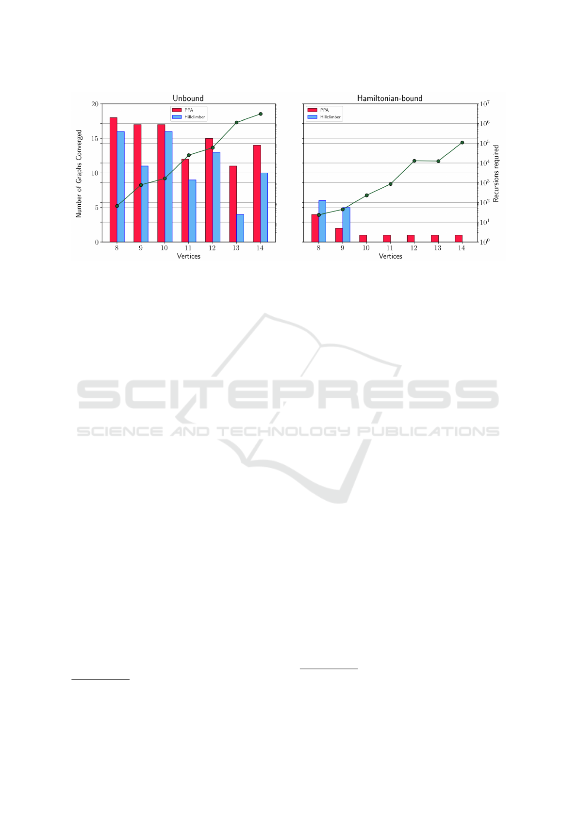
Figure 3: Recursions required for the hardest graph on the right-side vertical axis versus their corresponding graph size on
the horizontal axis. The left graph shows results of the experiment without restrictions on edge mutation, the right graph
shows the results of the experiment in which graphs forcibly retained an unmutable Hamiltonian cycle at all times. The bars
represent the number of multiple times a graph of maximum recursions was found.
through a public GitHub repository
4
.
3 EXPERIMENT
To obtain the hardest Hamiltonian cycle problem in-
stances, we evolve 560 graphs of sizes 8 ≤ V ≤ 14
in runs of 3000 evaluations. The investigation is
split in tow parts: an ’unbound’ experiment, in which
the evolutionary algorithms are free to modify all
the edges, and a ’Hamiltonian-bound’ experiment in
which the evolutionary algorithms are free to mod-
ify all the edges except the edges {(1, 2), (2, 3)...( v −
1,v), (v, 1)}, thereby enforcing the presence of a
Hamiltonian cycle in the graph at all times.
For the hillclimber runs, twenty randomly gener-
ated graphs were evenly dispersed in terms of edge
density, ranging from 0 to
1
/2V · (V − 1) edges, corre-
sponding to edge densities ∈ {0%,5%, 10%...100%}.
For the PPA runs, twenty initial populations were
made along the same edge density intervals, with
all graphs in one population having the same edge
density. It should be noted that these densities are
fixed only upon initialization, as the evolutionary al-
gorithms are free to insert and remove edges from
graphs at every step of a run. The rationale be-
hind these choices however, is that earlier results
could have been biased from the initialization on the
Koml
´
os-Szemer
´
edi bound. Besides, this approach
would cover more of the state space, at least as seen
from the initial conditions. In the end, it didn’t make
much of a difference.
4
https://github.com/Joeri1324/evolving-hard-hamilton-
cycles
From these evely distributed initial positions, both
algorithms ran for 3000 function evaluations. This
means 3000 iterations for the stochastic hillclimber,
but 120 generations of PPA, which produces 25 off-
spring, and therefore performs 25 evaluations per
generation (see Table 1). These numbers might
look small, as do the numbers of vertices in the
graphs used, but the number of recursions required
for Vacul’s solving algorithm in every function eval-
uation can still easily run in the millions (see Figure
3). And as we are actively pushing towards the max-
imum, the entire unbound experiment of 280 runs (7
graph sizes with 20 starting points for two evolution-
ary algorithms) with 3000 function evaluations still
took approximately 45 days on 16 cores of the LISA
cluster computer at Amsterdam’s Science Park
5
. The
280 runs of 3000 evaluations for the Hamiltonian-
bound experiment took significantly less time, possi-
bly because the Hamiltonian-bound instances require
significantly fewer recursions to decide. Hamilto-
nian instances are easier, generally speaking. But if
you want to see for yourself, all the experiment’s re-
sources are publicly available through a repository
6
.
5
https://userinfo.surfsara.nl/systems/lisa
6
https://github.com/Joeri1324/evolving-hard-hamilton-
cycles
ECTA 2020 - 12th International Conference on Evolutionary Computation Theory and Applications
44

Table 2: The smallest distance between the hardest and easiest problem instances for the Hamiltonian cycle problem is just
one bit: inserting an edge on either of the two possible insertion point types makes the hardest (non-Hamiltonian) instance
trivially Hamiltonian. Removing an edge from either of the three possible types will make for a (just slightly) easier non-
Hamiltonian instance. Only five one-bit operations are possible, due to the highly structured nature of the results. Instance
hardness is measured in number of recursions required by Vacul’s algorithm.
Graph size 8 9 10 11 12 13 14
Most difficult 67 785 1,673 25,061 61,051 1,139,785 3,091,141
Insert wall #1 8 9 10 11 12 13 14
Insert wall #2 8 - 10 - 12 - 14
Remove clique-clique 63 717 1,577 23,261 57,799 1,071,037 2,943,549
Remove wall-wall 49 - 1,081 - 47,655 - 2,016,877
Remove wall-clique 25 529 1,015 18,561 43,513 894,861 2,387,791
4 RESULTS
4.1 Unbound Experiment
The results of the unbound experiment clearly
show the hardest problem instances are all non-
Hamiltonian. Both evolutionary algorithms produced
structurally similar graphs consisting of a ‘clique’
and a ’wall’ for all vertex numbers (See Figure 1).
The clique is a fully connected subset consisting
of V
c(odd)
=
V −1
2
vertices in odd-sized graphs, and
V
c(even)
=
V −2
2
vertices in even-sized graphs. Every
graph of size V is a subgraph of size V + 1, even
though the exact addition of edges differs from odd
to even graphs. The edge number of these graphs is
consequently given by:
(V −V
c
) ·V
c
+
1
/2V
c
· (V
c
− 1) (3)
with V
c
= V
c(odd)
if V is odd, and
(V −V
c
) ·V
c
+
1
/2V
c
· (V
c
− 1) + 1 (4)
with V
c
= V
c(even)
if V is even. These quadratic
results suggest that the larger the graph, the further
away the hardest instances are from the Koml
´
os-
Szemer
´
edi bound, which only increases (double) log-
arithmically in V . It should be noted that these results
strongly contradict earlier findings that find the hard-
est instances close to the bound (Cheeseman et al.,
1991)(Culberson and Vandegriend, 2011). This might
be due to the random nature of the test sets, but for the
related SAT-problem, two studies led by Moshe Vardi
suggest that the hardness peak itself might also move,
depending on the specific solver used in the experi-
ments (Coarfa et al., 2000)(Aguirre and Vardi, 2001).
On the lognormal scale of Figure 3, the number
of recursions roughly follows a straight line with an
inclination of 0.78, indicating that for wall-and-clique
graphs of size V , the number of recursions increases
exponentially as approximately O(c
0.78V
), in which
c > 1. The number of required recursions wobbles a
bit in V , which is possibly due to discrepancy between
odd- and even-sized graphs. In the odd-sized graphs,
there are slightly more vertices in the clique, which
results in a higher edge density, and possibly more
required recursions.
In the unbound experiment, both the plant prop-
agation algorithm and the stochastic hillclimber con-
verged multiple times to the same graph. Hillclimber
between 4 and 16 out of 20 runs for each V , aver-
aging at about 11,3 (See the bars in Figure 3, left).
In its operation, the stochastic hillclimber is prone to
get stuck in local maxima, but the plant propagation
algorithm is well equipped for navigating large non-
convex search spaces with its highly mutative off-
spring at the bottom of the population. Maybe that’s
why the algorithm did solidly better however, with
an average of 14,9 out of 20 runs converging to the
(same) wall-and-clique graph, with all values between
11 and 18. It should be noted though, that PPA only
outperforms the hillclimber only after approximately
2000 evaluations, an effect that was also witnessed
in other problems (Geleijn et al., 2019). Because of
the consistent convergence through independent runs
of both algorithms, and the insensitivity of PPA to lo-
cal maxima, it seems possible that the wall-and-clique
graphs are indeed the hardest instances of the Hamil-
tonian cycle problem for Vacul’s algorithm. More-
over, this maximum appears to be connected through
a state path of monotonically increasing fitness val-
ues, but this yet awaits further verification. A slightly
eyebrow raising observation is that both algorithms
converge somewhat better for even numbers of V .
4.2 One-bit Neighbourhood
As an added bonus, the highly structured results of
the unbound experiment allow for an exhaustive map-
ping of the one-bit neighbourhood of the most diffi-
Looking for the Hardest Hamiltonian Cycle Problem Instances
45

Table 3: The edge-independent search space increases faster than exponential in the number of vertices, but the percentage
of Hamiltonian instances increases also. This results in an ever denser volume of Hamiltonian graphs, which might explain a
possible lack of convergence in the evolutionary algorithms for the Hamiltonian-bound experiment. Numbers are rounded.
Vertices 8 9 10 11 12 13 14
Graphs 2.68 ·10
8
6.87 ·10
10
3.52 ·10
13
3.60 ·10
16
7.38 ·10
19
3.02 ·10
23
2.48 ·10
27
Hamiltonian 57.9% 66.5% 74.4% 81.0% 86.3% 90.4% 93.4%
cult instances. For the odd-sized graphs, there is only
one possible graph type resulting from edge insertion.
For the even-sized graphs there are two neighbouring
graph types from inserting an edge, due to the ex-
tra edge in the wall. Both these edge insertions im-
mediately make the graph Hamiltonian and decidable
within V recursions (Table 2). It is a remarkable find-
ing, that the hardest non-Hamiltonian instances and
the easiest Hamiltonian instances are separated by just
one bit of information.
Removal of an edge can create two one-bit neigh-
bouring graph types in odd-sized graphs, either from
removal inside the clique, or removal of a wall-clique
edge. In even-sized graphs, a third removal is possi-
ble, from the single wall-wall edge. All edge removal
operations lower the number of recursions needed to
decide the graph, but the effect is much less dra-
matic than for inserting edges. Even though the num-
ber of recursions from edge removal drops between
6% and 63% for the smallest instances, the differ-
ence is only between 5% and 33% for the largest in-
stance in this study, and is expected to become ever
smaller for larger instances, simply because larger
graphs have more edges, so the removal of one could
have a smaller impact on recursion.
These neighbourhood results do show however,
that the wall-and-clique graphs are at the very least a
local maximum of instance hardness. But since both
algorithms repeatedly and independently converged
to the same graph, and PPA is not sensitive to lo-
cal maxima, it might well be that these graphs are
the hardest instances of the Hamiltonian cycle prob-
lem (for Vacul’s algorithm). These results could be
taken as a suggestion that harder problem instances
for the Vandegriend-Culberson algorithm do not ex-
ist, but more extensive testing could substantially
(dis)confirm this hypothesis.
4.3 Hamiltonian-bound Experiment
For the Hamiltonian-bound experiment, results are
much less unisono than for the unbound experiment.
The hardest Hamiltonian graphs found by the evolu-
tionary algorithms are still roughly a magnitude eas-
ier than the non-Hamiltonian graphs (See Figure 3,
right), with the number of recursions increasing as ap-
proximately O(c
0.62V
), in which c > 1. Again, this
exponent is a fit on only seven data points, needs fu-
ture refinement, but still serves as a rough indication.
The structural resemblance between graphs of dif-
ferent sizes is also much lower (Figure 2). For graphs
of size V = 8, the maximum number of recursions
was identical in two graphs, reached in 10 out of 40
runs. For V = 9, only 7 out of 40 runs reached any of
4 graphs with maximum recursions, and for larger V ,
the hardest Hamiltonian instance was unique among
40, with just a single PPA run producing that graph.
These results suggest that the hardest possible Hamil-
tonian instances might not yet have been found, and
that harder graphs are still possible. A neighbourhood
mapping was not done for these graphs, as the lack of
structure makes it relatively cumbersome, and results
inconclusive.
5 DISCUSSION
If the problem instances found in the unbound ex-
periment are indeed global maxima, it could indi-
cate that the problem space is largely convex, since
the stochastic hillclimber acquires similar results to
the PPA. In this sense, The wall-and-clique graph
might be sitting on the top of mount hardness, with
very easy Hamiltonian instances and very hard non-
Hamiltonian instances in its immediate vicinity. For
the Hamiltonian-bound experiment, such observa-
tions are less expedient, because convergence of the
algorithms appears unlikely. So what makes these al-
gorithms perform so bad on the Hamiltonian-bound
problem instances? Surely, less freedom from fix-
ing unmutable edges would make a problem easier,
right? The converse might actually be true, and the
argument is a somewhat bewildering and counterin-
tuitive numerical elaboration resulting from Koml
´
os
and Szemer
´
edi early results and some basic combina-
torics.
As presented in Equation 1, the probability of
a random graph being Hamiltonian sigmoidally de-
pends on the number of edges. But for a complete
edge independent search space such as ours, this prob-
ability might also be seen as a frequency. As a nu-
merical example: for V = 8 and E = 14, Koml
´
os and
Szemer
´
edi’s equations predict an approximate 61%
chance of Hamiltonicity. Equivalently, one could
say that 61% of all existable graphs with V = 8 and
ECTA 2020 - 12th International Conference on Evolutionary Computation Theory and Applications
46

E = 14 are Hamiltonian. Now the number of graphs
is equivalent to the number of options for placing the
E edges between V vertices:
1
/2 ·V · (V − 1)
E
(5)
which for V = 8 and E = 14, amounts to 40,116,600
graphs. Of these, approximately 61%, or 24,274,846
gaphs are Hamiltonian, the remaining 39%, or
15,841,754 graphs, are non-Hamiltonian. Summing
these results over all possible values of E for a given
V gives us the number (or percentage) of Hamiltonian
graphs in the entire edge-independent search space
(Table 3).
As it turns out, the number of Hamiltonian in-
stances ever more outweigh the number of non-
Hamiltonian instances as graphs get larger, possi-
bly making the state space harder to navigate for
our evolutionary algorithms, which have identical
numbers of evaluations for all V . This observation
might also account for the slightly deminishing re-
turns in both experiments for both algorithms as V
increases. But contrarily, these numbers do not ac-
count for graph isomorphism which might be quite
influential, but whose detection is a notorious prob-
lem in itself (McKay and Piperno, 2014). It is an
interesting and non-trivial question to see whether
other (meta)heuristic algorithms such as a properly
parameterized simulated annealing (Kirkpatrick et al.,
1983)(Dahmani et al., 2020) or genetic algorithms
(B
¨
ack et al., 1997) do better for this problem. It is also
plausible that metaheuristic parameter tuning and/or
control might set some serious sods to the dyke, as the
problem space clearly changes rapidly as V increases.
On a final note, these graphs might be difficult for
Vacul’s solving algorithm because its efficiency heav-
ily depends on pruning off edges that cannot be in
any Hamilton cycle, which only occurs when a vertex
is connected by two required edges. Because of the
compact structure of the wall-and-clique graph, this
will only happen near the full depth of the search tree,
when all but two vertices of the maximum clique are
included in a partial solution. But just the ubiquity of
pruning techniques throughout history doesn’t spell
much good for other exact algorithms either when
it comes to these graphs. The non-Hamiltonian in-
stances in this study might thereby actually be the
hardest around, but more evidence, or perhaps even
a proof, is needed to soldify this conjecture.
ACKNOWLEDGEMENTS
ECTA’s reviewers
7
really made an effort to under-
stand this somewhat pioneering approach to instance
hardness. A special hats off goes to Reviewer #4, who
took the time to hand-correct a host of typo’s and sup-
ply an annotated pdf along with the report. Thank you
all, you have done this paper a great favour.
REFERENCES
Aguirre, A. S. M. and Vardi, M. (2001). Random 3-sat and
bdds: The plot thickens further. In International Con-
ference on Principles and Practice of Constraint Pro-
gramming, pages 121–136. Springer.
B
¨
ack, T., Fogel, D. B., and Michalewicz, Z. (1997). Hand-
book of evolutionary computation. Release, 97(1):B1.
Br
´
elaz, D. (1979). New methods to color the vertices of a
graph. Communications of the ACM, 22(4):251–256.
Cheeseman, P., Kanefsky, B., and Taylor, W. M. (1991).
Where the really hard problems are. In Proceedings of
the 12th International Joint Conference on Artificial
Intelligence - Volume 1, IJCAI’91, pages 331–337,
San Francisco, CA, USA. Morgan Kaufmann Publish-
ers Inc.
Coarfa, C., Demopoulos, D. D., Aguirre, A. S. M., Sub-
ramanian, D., and Vardi, M. Y. (2000). Random 3-
sat: The plot thickens. In International Conference on
Principles and Practice of Constraint Programming,
pages 143–159. Springer.
Cook, S. A. (1971). The complexity of theorem-proving
procedures. In Proceedings of the Third Annual
ACM Symposium on Theory of Computing, STOC ’71,
pages 151–158, New York, NY, USA. ACM.
Culberson, J. C. and Vandegriend, B. (2011). The gn,m
phase transition is not hard for the hamiltonian cycle
problem. CoRR, abs/1105.5443.
Dahmani, R., Boogmans, S., Meijs, A., and van den Berg,
D. (2020). Paintings-from-polygons: simulated an-
nealing. In International Conference on Computa-
tional Creativity (ICCC’20).
de Jonge, M. and van den Berg, D. (2020). Plant propa-
gation parameterization: Offspring & population size.
Evo* 2020, page 19.
Garey, M. R. and Johnson, D. S. (1990). Computers
and Intractability; A Guide to the Theory of NP-
Completeness. W. H. Freeman & Co., New York, NY,
USA.
Geleijn, R., van der Meer, M., van der Post, Q., and van den
Berg, D. (2019). The plant propagation algorithm on
timetables: First results. EVO* 2019, page 2.
Held, M. and Karp, R. M. (1962). A dynamic program-
ming approach to sequencing problems. Journal of
the Society for Industrial and Applied mathematics,
10(1):196–210.
7
ECTA 2020 is part of the larger conference IJCCI 2020,
see http://www.ecta.ijcci.org/.
Looking for the Hardest Hamiltonian Cycle Problem Instances
47

Hutter, F., Xu, L., Hoos, H. H., and Leyton-Brown, K.
(2014). Algorithm runtime prediction: Methods &
evaluation. Artificial Intelligence, 206:79–111.
Karp, R. M. (1972). Reducibility among combinatorial
problems. In Miller, R. E., Thatcher, J. W., and
Bohlinger, J. D., editors, Complexity of Computer
Computations: Proceedings of a symposium on the
Complexity of Computer Computations, held March
20–22, 1972, at the IBM Thomas J. Watson Re-
search Center, Yorktown Heights, New York, and spon-
sored by the Office of Naval Research, Mathemat-
ics Program, IBM World Trade Corporation, and the
IBM Research Mathematical Sciences Department,
Boston, MA. Springer US.
Kirkpatrick, S., Gelatt, C. D., and Vecchi, M. P. (1983).
Optimization by simulated annealing. science,
220(4598):671–680.
Koml
´
os, J. and Szemer
´
edi, E. (1983). Limit distribution for
the existence of hamiltonian cycles in a random graph.
Discrete Mathematics, 43(1):55–63.
Larrabee, T. and Tsuji, Y. (1993). Evidence for a satisfia-
bility threshold for random 3cnf formulas. Technical
report.
Li, M., Vit
´
anyi, P., et al. (2008). An introduction to Kol-
mogorov complexity and its applications, volume 3.
Springer.
Martello, S. (1983). Algorithm 595: An enumarative al-
gorithm for finding hamiltonian circuits in a directed
graph.
McKay, B. D. and Piperno, A. (2014). Practical graph
isomorphism, ii. Journal of Symbolic Computation,
60:94–112.
Paauw, M. and Van den Berg, D. (2019). Paintings,
polygons and plant propagation. In International
Conference on Computational Intelligence in Music,
Sound, Art and Design (Part of EvoStar), pages 84–
97. Springer.
Rubin, F. (1974). A search procedure for hamilton paths
and circuits. J. ACM, 21(4):576–580.
Salhi, A. and Fraga, E. S. (2011). Nature-inspired optimi-
sation approaches and the new plant propagation algo-
rithm.
Selamo
˘
glu, B.
˙
I. and Salhi, A. (2016). The plant propaga-
tion algorithm for discrete optimisation: The case of
the travelling salesman problem. In Nature-inspired
computation in engineering, pages 43–61. Springer.
Selman, B., Mitchell, D. G., and Levesque, H. J. (1996).
Generating hard satisfiability problems. Artificial In-
telligence, 81(1):17 – 29. Frontiers in Problem Solv-
ing: Phase Transitions and Complexity.
Sleegers, J. and van den Berg, D. (2020). Plant propagation
& hard hamiltonian graphs. Evo* 2020, page 10.
Tarjan, R. (1972). Depth-first search and linear graph algo-
rithms. SIAM journal on computing, 1(2):146–160.
Turner, J. S. (1988). Almost all k-colorable graphs are easy
to color. Journal of Algorithms, 9(1):63 – 82.
van Horn, G., Olij, R., Sleegers, J., and van den Berg, D.
(2018). A predictive data analytic for the hardness of
hamiltonian cycle problem instances. DATA ANALYT-
ICS 2018 : The Seventh International Conference on
Data Analytics.
Vrielink, W. and van den Berg, D. (2019). Fireworks algo-
rithm versus plant propagation algorithm.
ECTA 2020 - 12th International Conference on Evolutionary Computation Theory and Applications
48
