
A Visual Intelligence Scheme for Hard Drive Disassembly in Automated
Recycling Routines
Erenus Yildiz
1 a
, Tobias Brinker
1 b
, Erwan Renaudo
2 c
, Jakob J. Hollenstein
2 d
,
Simon Haller-Seeber
2 e
, Justus Piater
2 f
and Florentin Wörgötter
1 g
1
III. Physics Institute, Georg-August University of Göttingen, Germany
2
Department of Computer Science, University of Innsbruck, Innsbruck, Austria
Keywords:
Object Detection, Object Classification, Automation, e-Waste, Recycling.
Abstract:
As the state-of-the-art deep learning models are taking the leap to generalize and leverage automation, they
are becoming useful in real-world tasks such as disassembly of devices by robotic manipulation. We address
the problem of analyzing the visual scenes on industrial-grade tasks, for example, automated robotic recycling
of a computer hard drive with small components and little space for manipulation. We implement a supervised
learning architecture combining deep neural networks and standard pointcloud processing for detecting and
recognizing hard drives parts, screws, and gaps. We evaluate the architecture on a custom hard drive dataset
and reach an accuracy higher than 75% in every component used in our pipeline. Additionally, we show that
the pipeline can generalize on damaged hard drives. Our approach combining several specialized modules can
provide a robust description of a device usable for manipulation by a robotic system. To our knowledge, we
are the pioneers to offer a complete scheme to address the entire disassembly process of the chosen device. To
facilitate the pursuit of this issue of global concern, we provide a taxonomy for the target device to be used in
automated disassembly scenarios and publish our collected dataset and code.
1 INTRODUCTION
Today’s electronic products have a short life cycle,
as they are usually discarded before their materials
degrade. Studies like (Duflou et al., 2008) showed
that 1) the recycling processes of these products are
mostly done by humans, 2) even when automated, the
processes are usually destructive – leading to the loss
of valuable metals and rare earth materials (Tabuchi,
2010; Massari and Ruberti, 2013). There is thus a
strong need for less-destructive recycling processes,
as illustrated by a recent initiative to reuse magnets
from retired hard-disk drives (HDD) in order to re-
duce the demand on rare earth materials
1
. In addition,
the hazardous elements used in electronic products
a
https://orcid.org/0000-0002-3601-7328
b
https://orcid.org/0000-0003-2930-158X
c
https://orcid.org/0000-0003-3282-8972
d
https://orcid.org/0000-0001-5694-691X
e
https://orcid.org/0000-0002-1538-5906
f
https://orcid.org/0000-0002-1898-3362
g
https://orcid.org/0000-0001-8206-9738
1
https://spectrum.ieee.org/energywise/energy/environment/
making-new-hard-disk-drives-from-recycled-magnets
(e.g. Beryllium in GSM amplifiers) pose a threat to
the health of employees due to their carcinogenic na-
ture. Even with enforced security measures, avoiding
exposure of humans to such substances is paramount.
Thus, there are both health and economical reasons to
improve automation of the disassembly and recycling
processes.
From a robotics perspective, the disassembly pro-
cess presents a high automation potential due to its
repetitiveness. However great adaptability of such a
system is required, as EOL products to be recycled
can be of various nature (from house-office equip-
ment to entertainment, communication, etc.) or they
might be partially damaged. Moreover, some de-
vices within the same family of products present a
high intra-class variance of their parts’ shape depend-
ing on their brand or model. These variances im-
plies that a robotic disassembly system can not rely
on an open-loop procedure but has to analyze the
product to find the best disassembly strategy. It thus
needs efficient perception capabilities to provide rel-
evant information to the rest of the system. Several
parameters must be extracted from the scene: prod-
uct’s parts must be identified from the sensor data
Yildiz, E., Brinker, T., Renaudo, E., Hollenstein, J., Haller-Seeber, S., Piater, J. and Wörgötter, F.
A Visual Intelligence Scheme for Hard Drive Disassembly in Automated Recycling Routines.
DOI: 10.5220/0010016000170027
In Proceedings of the International Conference on Robotics, Computer Vision and Intelligent Systems (ROBOVIS 2020), pages 17-27
ISBN: 978-989-758-479-4
Copyright
c
2020 by SCITEPRESS – Science and Technology Publications, Lda. All rights reserved
17

and their pose must be estimated to allow the robot
to interact with the device. Sensors of various types
can be used (precise laser scanner, etc. (Weigl-Seitz
et al., 2006)), however vision sensors offer the best
cost/performance/adaptability solution given the tasks
to complete. In this work, we thus introduce a vision-
based perception scheme capable of analyzing a prod-
uct at different stages of disassembly. We evaluate it
on one class of undamaged devices, computer hard
drives (HDDs), which are one of the most common
devices encountered in E-Waste, and suitable in size
for robotic manipulation. This paper is organized as
follows: Section 2 gives a review of the literature
on vision-based methods, Section 3 presents our ap-
proach in detail, Section 4 presents the evaluation of
the method on the target device. Section 5 discuss the
impact of these results and concludes.
2 RELATED WORK
Computer vision techniques have been extensively
applied to industrial applications, e.g. defect detec-
tion, part recognition, etc. (Bi and Wang, 2010; Mala-
mas et al., 2003). However, not much work is done
in the context of automated recycling, where multi-
ple valuable parts must be identified for recovery. A
short survey of existing approaches in 2006 (Weigl-
Seitz et al., 2006) showed numerous limitations also
found in later work. First the focus on detecting a
specific class of component to detect – e.g. screws
((Bdiwi et al., 2016; Ukida, 2007; Bailey-Van Kuren,
2002), bolts (Wegener et al., 2015) – reduces the
generality of the method and its applicability in the
context of recycling where several types of compo-
nents must be gathered. The use of fully model-
based methods (Elsayed et al., 2012; Xie et al., 2008;
Ukida, 2007; Pomares et al., 2004; Torres et al., 2003;
Tonko and Nagel, 2000) implies the availability of
(e.g. CAD) models. This is a strong assumption as
these models are rarely available for every brand and
every type of device. Moreover, the recycling do-
main does not guarantee that devices are in an in-
tact state. Finally, another important limitation is
the use of non-adaptive feature detection techniques
(Bdiwi et al., 2016; Wegener et al., 2015; Weigl-Seitz
et al., 2006; Bailey-Van Kuren, 2002; Karlsson and
Järrhed, 2000). As mentioned previously, the high
intra-class and inter-brand variances of components
reduces the relevance of a human-engineered descrip-
tor of a component class. This limitation is only par-
tially explained by the date of publication of some
works (Weigl-Seitz et al., 2006; Bailey-Van Kuren,
2002; Karlsson and Järrhed, 2000).
On one hand, it seems that there is still a substan-
tial lack in generalizable, device and environment-
independent methods, which can be used in disassem-
bly processes. On the other hand, Deep Convolutional
Neural Networks (DCNN) offer a powerful solution
to analyze the inner structure of devices in the context
of disassembly. These methods have the potential to
solve the problems highlighted before: the specificity
of a detector can be tackled by training on a dataset
that includes samples of multiple parts of the targeted
device (and extended by retraining later on) and thus
being able to recognize these parts in all the devices
that use them. The lack of adaptability is addressed
by the nature of deep networks: as machine learn-
ing methods, they are problem and feature agnostic
before training. Finally most of these methods are
CAD model-free, meaning that they do not require
device-specific description sheets. They learn the rel-
evant features of a part class by themselves, abstract-
ing from the details of a specific brand and model. In
E-Waste recycling context, devices found in the same
family of devices often include similar parts such as
PCBs, screws, wires, etc. Extracting features from
these using visual paradigms usually leads to repro-
ducible results that can be used and further developed
for other devices as well.
Thus, the problem of disassembly scene analysis
can be formulated as a problem where machine learn-
ing paradigms (e.g. segmentation, classification) and
traditional data (e.g. pointcloud) analysis methods are
used in order to recognize the present parts of the tar-
get device. In contrast to other application domains,
the context of recycling E-Waste adds the following
constraints:
• The position estimation of parts must be precise
enough to allow manipulation of small parts in the
device.
• There is a strong degree of occlusion because
parts are intertwined, e.g. the platters and R/W
head of a hard drive.
• There is substantial intra-class variance for spe-
cific parts depending on the device brand or model
or the potential damage of the part.
The Semantic Segmentation problem (also known
as pixelwise classification problem) has been ad-
dressed in domains ranging from autonomous driv-
ing, human-computer interaction, to robotics, medi-
cal research, agriculture (Li et al., 2017; Dai et al.,
2016; Liu et al., 2018; Fu et al., 2019; Lin et al.,
2019; Dvornik et al., 2017). However, to the best
of our knowledge, no work currently address the do-
main of automated recycling of E-Waste. In these
domains, the state-of-the-art performance is achieved
ROBOVIS 2020 - International Conference on Robotics, Computer Vision and Intelligent Systems
18

using deep learning methods, especially Convolu-
tional networks (CNNs or ConvNets) (Krizhevsky
et al., 2012). Fully Convolutional Networks (FCN)
have been the standard algorithm to achieve pixelwise
segmentation of images (Badrinarayanan et al., 2017;
Long et al., 2015; Ronneberger et al., 2015) in vari-
ous domains such as medicine, autonomous driving,
domestic robotics. They extend CNN by replacing
fully-connected layers by convolutional layers, allow-
ing for arbitrary-sized input with no need for region-
proposal. The trade-off however, due to the nature of
the layers, is that the prediction of boundaries lacks
precision. This problem is addressed by a set of im-
provement to the networks (e.g. multi-resolution ar-
chitecture with skip connections (Ghiasi and Fowlkes,
2016; Lin et al., 2017a), mask refinement (Pinheiro
et al., 2016)). Additionally, pixelwise segmentation
requires labeled data which has a higher cost of pro-
duction (Lin et al., 2014). Weakly-supervised meth-
ods have been developed to tackle this issue (Zhang
et al., 2019): these methods iterate between learn-
ing using coarse bounding boxes as labels then refin-
ing them into more precise masks (Dai et al., 2015;
Khoreva et al., 2017). They achieve similar perfor-
mance as fully supervised methods at a lower la-
belling cost. Another main approach is called Region-
Based Semantic Segmentation. This method relies
on a pre-processing of the input image into candidate
objects (region proposals) for which features are ex-
tracted. These features are then used for the classifi-
cation. There is an entire family of R-CNN networks
(Girshick et al., 2014; Girshick, 2015; Ren et al.,
2015) that have been evolving and finally the cur-
rent state-of-the-art networks of the family is called
Mask-RCNN (He et al., 2017) which is based on
Feature Pyramid Network (FPN) (Lin et al., 2017b).
Mask-RCNN has been used by Facebook AI Research
(Joulin et al., 2016) as well as by medicine studies
(Johnson, 2018; Couteaux et al., 2019; Chen et al.,
2019).
Mask-RCNN and its ensembled models are cur-
rently the state of the art for object detection and in-
stance segmentation, and the reason for this is the
region-based detection mechanism mentioned earlier.
The core idea behind Mask-RCNN is to scan over the
predefined regions called anchors. RPN, then, does
two different types of predictions for each anchor.
First is the score of the anchor being foreground, and
the bounding box regression. The fixed number of
anchors with the highest score are then chosen, and
the regression adjustment is applied to get the final
proposal for object prediction at the network head.
There are other architectures that could be used for
this very task, such as the ensembled model Cascade-
RCNN (Cai and Vasconcelos, 2018). Through the ex-
perimental evaluation we conducted in Section 4, we
found out that Mobile-RCNN (Howard et al., 2017)
works better for our domain.
3 METHODS
Our visual scheme outputs on request a scene anal-
ysis that combines the predictions of 3 modules: a
part detection module, a screw detection module and
a gap detection module. The part detection module
recognizes most inner components of electronic de-
vices (HDD in our case). A specialized screw detec-
tor module detects various screw types as a separate
task from the part detection. Finally, gaps are also de-
tected as they provide useful information for robotic
manipulation of parts and tool. The pseudo code for
the pipeline is given in algorithm 1.
As mentioned earlier, the analysis of parts is a
semantic segmentation problem, but the screw de-
tection can be simplified as a classification problem:
rather than trying to find screws boundaries, we make
the hypothesis that they are mostly circular structures
in the scene. The new problem is thus to classify
detected circles in the image as screws or artefacts
(holes, stickers, etc.), with a specialized network.
3.1 Taxonomy & Datasets
In order to train the different modules of our pipeline,
we collect and create datasets. The first step is to
define a taxonomy of the HDD, which is done in
agreement with an industrial partner providing hard-
ware samples and data. The taxonomy provides the
class labels and is available on the IMAGINE web-
site
2
. Two datasets are created (a) for parts and (b)
for screws. For (a), top-down views of the computer
hard drives are annotated into 12 classes correspond-
ing to parts of interest according to the taxonomy. 500
images of 7 different brands (Hitachi, IBM, Maxtor,
Seagate, WD, Samsung, Toshiba) and models are col-
lected under different light conditions. These images
include various stages of disassembly with parts in ar-
bitrary positions (e.g. after a failed action). 5% of all
images correspond to damaged devices to account re-
alistically for the state of products in recycling plants.
The dataset is split into a validation set (10% of the
images), a test set (10%) and a training set (80%).
For (b), 10700 samples are annotated into 23% of
screws and 77% of artifacts. The training set includes
1491 screws and 4924 artifacts. The test set includes
2
https://imagine-h2020.eu/hdd-taxonomy.php
A Visual Intelligence Scheme for Hard Drive Disassembly in Automated Recycling Routines
19
Algorithm 1: Perception Pipeline.
1: c
p
, b
p
, m
p
:= [] part centers, boundaries, masks
2: c
s
, b
s
, m
s
:= [] screw centers, boundaries, masks
3: c
g
, b
g
, v
g
:= [] gap centers, boundaries, volumes
4: I, P := NULL I: Input Monocular Image, P: Input Pointcloud
5: C
m
,C
s
:= NULL C
m
: Monocular Calibration Info, C
s
: Stereo Calibration Info
6: predicates = []
7: procedure COLLECT PREDICATES
8: if hddTable.State() = 0 then
9: hddTable.changeState(angle = θ
Stereo
)
10: P := getPointcloud(P)
11: if P 6= NU LL then
12: c
g
, b
g
, v
g
← detectGaps(P)
13: hddTable.changeState(angle = θ
Monocular
)
14: I := getRGBImage(I)
15: if I 6= NULL & hddTable.State() = 0 then
16: c
p
, b
p
, m
p
← segmentParts(I)
17: c
s
, b
s
, m
s
← detectScrews(I)
18: C
m
,C
s
← getCalibrationIn f o()
19: predicates := mergeAllIn f o(I, P,C
m
,C
s
, c
p
, b
p
, m
p
, c
s
, b
s
, m
s
, c
g
, b
g
, v
g
)
20: return predicates
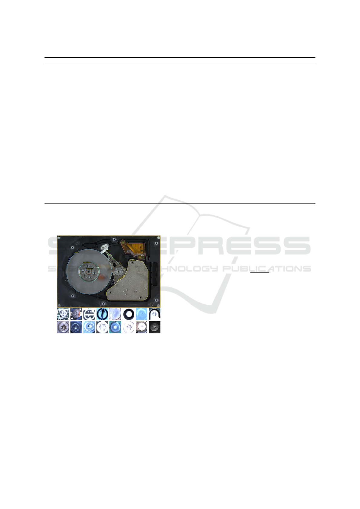
1000 screws and 3285 artifacts. Figure 1 illustrates
an annotated drive (top) and a sample of artefacts and
screws found during the disassembly (bottom).
Figure 1: Top: Ground truth annotations for a sample hard
drive based on the taxonomy, used for part segmentation
task (above). Bottom: Training dataset containing (first
row) artefacts and (second row) screws for the detection of
screws.
3.2 Part Segmentation
We address the semantic segmentation problem with
Deep CNNs to detect, recognize and localize the inner
parts of the device. Due to the high number of avail-
able state-of-the-art networks, we train and evaluate
a set of selected methods on this instance segmenta-
tion problem: MobileNetV1 (Howard et al., 2017),
MobileNetV2 (Sandler et al., 2018), Cascade-RCNN
(Cai and Vasconcelos, 2018), native Mask-RCNN
(He et al., 2017), and finally the ensembled model of
Cascade-MobileNetV1 . All networks were trained
with data augmentation turned on as suggested by the
native Mask-RCNN authors, we apply the same aug-
mentation procedures. The accuracy of a network is
computed using the similarity IoU metric (see eq. 1):
IoU =
| A ∩ B |
| A ∪ B |
(1)
where A and B are respectively the sets of pre-
dicted and ground truth bounding boxes. The results
of this preliminary study are available in Table 1. Al-
though Cascade-RCNN obtains the best segmentation
results, we selected Mobile-RCNN that comes right
after, since the model is lighter, and, thus, it is em-
ployed in the part detection module of our architec-
ture.
3.3 Screw Detection
The screw detection module classifies potential candi-
dates input into the screw or artefact classes. We inte-
grate the algorithm presented in (Yildiz and Wörgöt-
ter, 2019) into our pipeline. We describe the algo-
rithm briefly hereafter and refer the reader to the pub-
lication for an extended description and analysis.
The algorithm combines classical vision prepro-
cessing of the input image with deep learning meth-
ods for classification. The image is processed with
the Hough circle transform (Duda and Hart, 1971) to
generate screw candidates as local views of the in-
ROBOVIS 2020 - International Conference on Robotics, Computer Vision and Intelligent Systems
20

Table 1: IoU values of different networks evaluated on our test set. Cascade-RCNN and MobV1-RCNN seem to be the best
performing ones.
DCNN Identifier Cascading Backbone AP AP
0.5
AP
0.75
AP
s
AP
m
AP
l
Mean-F
Mask-RCNN No ResNet-101-FPN 41.2 65.7 47.6 16.3 42.3 42.4 0.70
MobV1-RCNN No Mobilenetv1-224-FPN 56.2 76.7 64.9 20.6 54.6 59.7 0.78
MobV2-RCNN No Mobilenetv2-FPN 34.6 60.5 35.5 3.8 15.4 43.6 0.63
Cas-Mob-RCNN Yes Mobilenetv1-224-FPN 28.5 43.3 33.3 20.0 13.3 35.4 0.61
Cas-RCNN Yes ResNet-101-FPN 61.3 76.4 72.6 35.1 61.8 65.4 0.84
put image. These candidates are sent to an ensemble
of two networks (InceptionV3 (Szegedy et al., 2016)
and Xception (Chollet, 2017) both with an additional
dropout layer before their last fully-connected layer)
and their output are combined through a weighted
sum. The network finally output its prediction on
the nature of the candidate (screw or artifact). The
method is reported to achieve a 99% successful clas-
sification rate (Yildiz and Wörgötter, 2019).
The most significant feature of this work is clearly
its adaptation ability. Since we are proposing a visual
scheme for disassembly processes, we must consider
the fact that our target device (HDD) is not going to
be the only device to be disassembled for long. Since
the chosen screw detection paradigm already works
well for the screws encountered in hard drives, along
with the fact that it allows users to collect new datasets
very quickly, we are sure of its adaptability even if the
target device or the environment changes at a point.
We’ve experimented with the integrated screw de-
tection module and we share its results in Section 4.
3.4 Position Estimation
The part detection and screw detection module oper-
ate only on RGB image data. To act on the detected
screws and parts, their pixel coordinates (2D) need to
be related to positions in the robot’s frame (3D). We
will refer to this process as localization. We use an
RGB-D camera to get a point-cloud representation of
the scene and relate pixels to points (see Figure 3 for
the relative poses of the camera). The correspondence
is done by projecting the point-cloud points into pixel
coordinates, and estimating a k-nearest-neighbor re-
gressor to perform the inverse operation: mapping
pixels to 3D positions. This process is repeated each
time the scene analysis is performed, i.e. upon request
from the rest of the system. These requests come
asynchronously at less than 1 Hz thus there are no
time constraint in this case.
3.5 Gap Detection
The gap detection relies on the top-view point-cloud
representation of the scene acquired by the stereo
camera. The overall process along sample views for
each step is presented in Figure 2. The point-cloud
is processed by a passthrough filter to find the re-
gion of interest: points outside a volume (i.e. box-
shaped) in which the HDD should be positioned are
discarded to remove artifacts. The output point-cloud
is then denoised: We are using sparse outlier removal
(Rusu et al., 2008), which identifies outlier points
based on their mean distance to their nearest neigh-
bours. The denoised point-cloud depth distribution
is then analysed to classify the points into surface
points and gap points. Because the existence of gaps
produces a bi-modal depth distribution between fore-
ground points (surface) and background points (gaps),
a simple threshold can be computed automatically
(e.g. using (Otsu, 1979)). The candidate gap points
are then clustered into separate gaps using a density-
based clustering approach (DBSCAN with manually
set parameters). This step provides the location and
size of the gaps and excludes the spaces too small to
be interesting gaps. In order to extrapolate the volume
of each gap, a convex hull algorithm is used to get the
2D boundaries of the gap in a first pass. Then arti-
ficial points are added to each cluster by duplicating
the boundary points and setting their height to the me-
dian height of the surface points identified earlier. A
second pass of the convex hull algorithm provides the
corrected 3D gap volumes, which are then filtered to
remove very small volumes. The gap centers are esti-
mated as the mean of the extrema for every axis. The
set of found gaps including their centers and volumes
are sent back to the rest of the pipeline.
4 RESULTS
4.1 Experiments
4.1.1 Setup
Our visual scheme requires two inputs: a top-down
RGB image and a top-down point-cloud. We built an
automated system that uses a tilting table holding the
device either horizontal (its surface normal aligned
with the RGB camera) or 45
◦
(aligned with the RGB-
A Visual Intelligence Scheme for Hard Drive Disassembly in Automated Recycling Routines
21
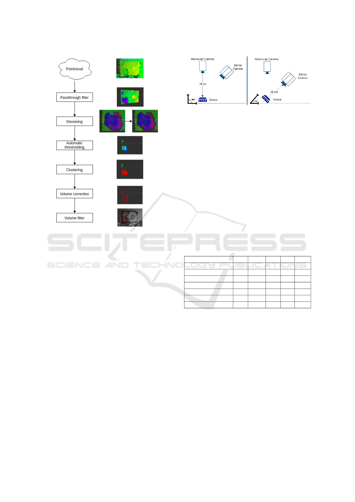
Figure 2: Complete pipeline for the gap detection module.
Initially, a passthrough filter discards the points below the
lower limit and points above the upper limit for the specified
axis. The noise created from the stereo cameras is removed
via sparse outlier removal (Rusu et al., 2008). Following,
thresholding is done only on the Z-axis since it denotes the
height of the points in the cloud. Deeper points are very
likely to belong to a gap, therefore, using a well-chosen
threshold we can split the point cloud based on the depth
of points into potential gap points and insignificant surface
points. Points belonging to a gap often lie in close proxim-
ity to each other, opening an opportunity for a clustering ap-
proach (DBSCAN, HDBSCAN) to label points. A volume
correction is applied by adding artificial points to the set of
gap points, so that the convex hull algorithm uses them as
the new outline points and creates a better estimate. As a
last step, the volume filter is used to throw away extremely
small volumes that cannot be gaps given the device’s natural
shape.
D stereo camera) on request (see Figure 3). We use
a Basler acA4600-7gc monocular camera which pro-
vides images with 4608 × 3288 resolution and 3.5
FPS and a Nerian Karmin2 stereo camera with a depth
error of 0.06cm from the minimum range of 35cm.
4.2 Evaluation Method
There are three main blocks in our scheme and each
of these blocks has to be evaluated differently, as the
paradigms running behind are different. Evaluation
of the screw detection used was already conducted in
Figure 3: Setup used for evaluation: a monocular RGB
camera is oriented downwards (θ
Monocular
= 90
◦
) and a
stereo RGB-D camera is mounted at θ
Stereo
= 45
◦
. This
configuration is due to the different focal lengths of the cam-
eras. Both are pointing at the device to be analysed. A
tilting mechanism allows the system to obtain “top-down”
views of the devices with both cameras.
its paper, thus, the results are directly taken from that
work (Yildiz and Wörgötter, 2019). For part segmen-
tation, we are going to go by the IoU (Intersection
over Union) metric and report the AP, as it has become
the de facto evaluation metric for instance segmenta-
tion networks. One very similar work was recently
evaluated the same way (Jahanian et al., 2019). Fi-
nally the gap detection is evaluated with a metric that
we came up ourselves, which we are going to discuss
in its respective subsection.
4.2.1 Screw Detection
Table 2: Classifier accuracy of different state-of-the-art net-
works, from (Yildiz and Wörgötter, 2019) with permission.
Model TP TN FP FN Acc
Xception 975 3244 25 41 98.5
InceptionV3 973 3262 27 23 98.8
ResneXt101 962 3260 38 25 98.5
InceptionResnetV2 965 3260 35 25 98.6
DenseNet201 897 3272 103 13 97.3
ResNetV2 943 3208 57 77 96.9
Integrated model 988 3254 12 31 99.0
We first would like to report the classifier accuracy in
Table 2 which are directly taken from the work (Yildiz
and Wörgötter, 2019) published. However, although
the classifier accuracy is quite high, due to the fact
that Hough circle finder method misses out finding
the circles in the first place, our final average precision
was found to be 80%. As the classifier expects images
that are directly suggested by the Hough circle finder,
any circle that is missed, is also not considered by
the classifier. In other words, the classifier’s ability is
limited by the Hough circle finder. Therefore, the AP
remains at 80%. We refer the reader to the Figure 4
to illustrate a few detection samples during the HDD
disassembly sequences.
ROBOVIS 2020 - International Conference on Robotics, Computer Vision and Intelligent Systems
22
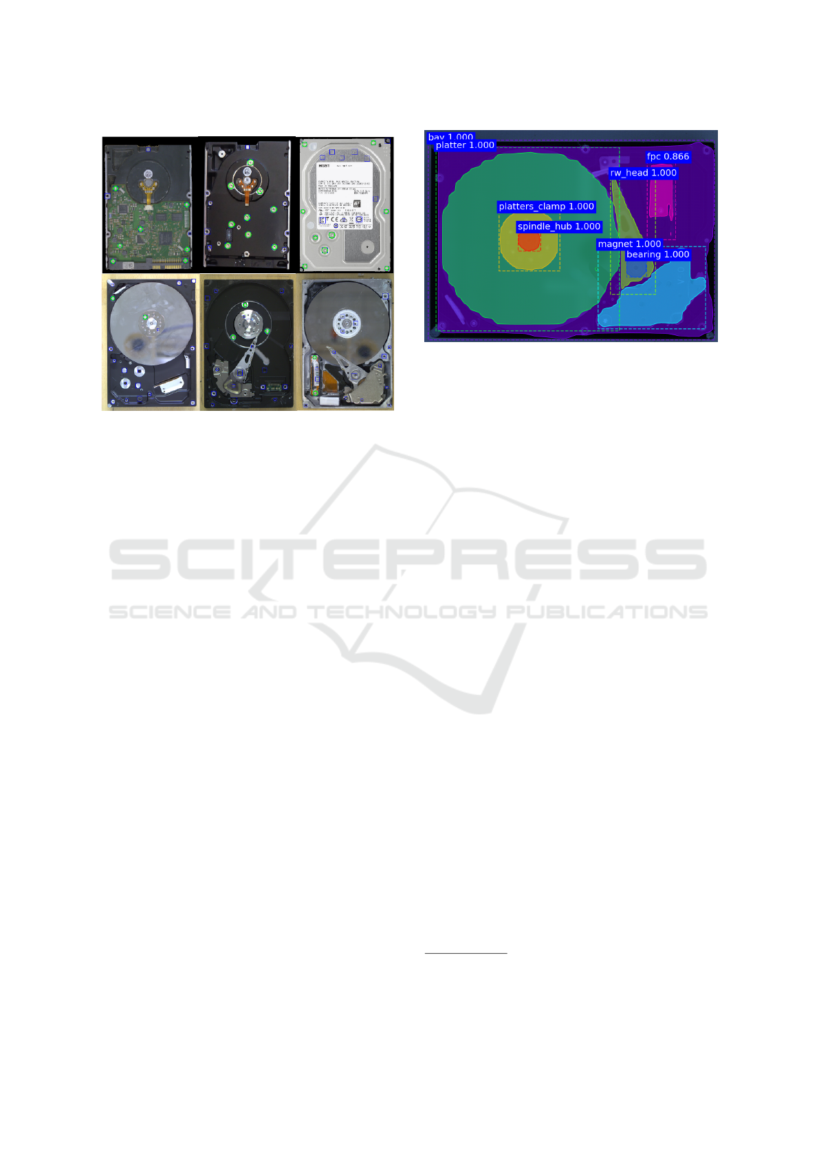
Figure 4: Outputs from the integrated screw detection mod-
ule. Blue circles highlight the candidates suggested by the
Hough circle finder, whereas green circles are the detected
screws by the model taken from a study (Yildiz and Wörgöt-
ter, 2019).
4.2.2 Part Segmentation
As mentioned earlier, the standard metrics for pixel to
pixel segmentation are mainly the COCO (Lin et al.,
2014) average precision (AP) metrics: AP is aver-
age precision of multiple IoU values. As reported
in Table 1, MobV1-RCNN and CAS-RCNN achieve
the best segmentation performances (resp. 0.78 and
0.84). These results are achieved after 500 epochs of
training on Google Colaboratory (Bisong, 2019) envi-
ronment using Tensorflow (Abadi et al., 2016) 1.15.2.
Figure 5 shows a sample output of the part segmenta-
tion process.
From our experiments, we make the following
conclusions. MobileNetV2 has stabilization issues
since the model is not able to predict on every scene
after a certain amount of training. We observed in the
training history that the loss becomes undetermined
and thus the model remains unstable. It could be ar-
gued that the reason is the dataset, i.e. the classes are
not uniformly distributed. On the other hand, cascad-
ing lighter backbones such as MobileNetV1 does not
ensure better feature extraction property. In fact, our
modeling suggests that it actually decreases efficiency
due to usage of depthwise convolutions. However,
this situation in return, validates the choice of back-
bone with residual nets that is clearly done in the orig-
inal CBNet (Liu et al., 2019), Cascade-RCNN (Cai
and Vasconcelos, 2018). In short, we find out that
cascading should only be done with models that has
residual backbones such as ResNet and its variants.
Figure 5: Output of the part segmentation module powered
by MobV1-RCNN. Each color represents a different part
predicted by the network whose names and prediction val-
ues are given. In this case, all parts and boundaries are cor-
rectly detected.
During our investigations we noticed that increasing
cascading with more detection target and logits loss
destabilizes the model. The use of DenseNet (Huang
et al., 2016) may increase accuracy, however, with
non-distributed class data like ours, stabilization re-
mains an issue. This is due to the fact that the last
layers in the network cannot handle class-logits when
the feature data is non-distributed. In the presence
of multi-GPU systems, we recommend ResNext-152
(Xie et al., 2017) to be investigated for higher accu-
racy.
Instead of selecting Cascade-RCNN, we made our
choice with MobV1-RCNN due to the fact that it re-
mains stable in the presence of high resolutions, un-
like Cascade-RCNN that is unstable despite of having
high accuracy. Since our setup uses high-resolution
images, we therefore employed MobV1-RCNN as our
final model in the segmentation scheme. However, for
future reference, we note that combining images of
different resolutions in a dataset creates problems in
stable models as the model is not stable during train-
ing.
4.2.3 Gap Detection
In order to evaluate the performance of the gap de-
tector, we had to create ground truth. To this end, all
point clouds taken by the stereo cameras were anno-
tated using a Semantic Segmentation Editor
3
. These
ground truth annotations consist of point wise seg-
mentations of each gap in a device. To get comparable
point numbers, sparse outlier denoising was run on
the clouds before segmentation. Based on the found
3
https://github.com/Hitachi-Automotive-And-Industry-Lab/
semantic-segmentation-editor
A Visual Intelligence Scheme for Hard Drive Disassembly in Automated Recycling Routines
23
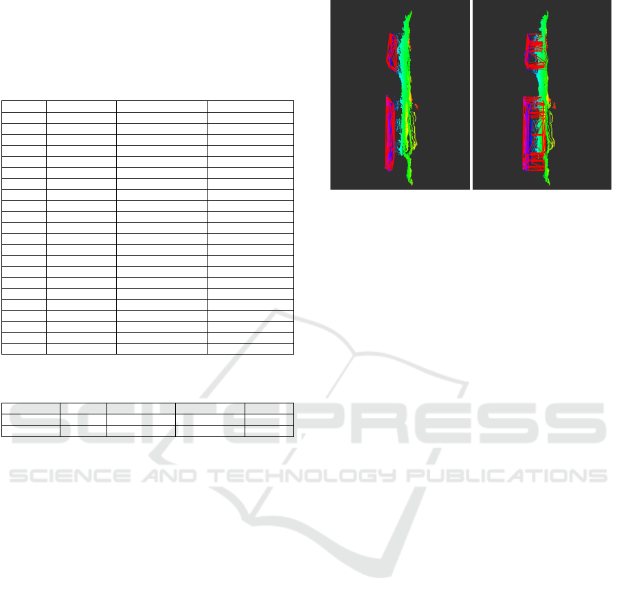
Table 3: Comparison of the DBSCAN powered detector’s
output and the ground truth annotations. Mean error is
found to be 24.30% among the identified gaps. Gaps that
were not identified due to the shortcomings of the sensor
were left out of the calculation. These are the gaps that are
usually extremely small and irrelevant to the disassembly
routine.
Detected (cm
3
) Ground Truth (cm
3
) Error(%)
Gap #1 36.3 46.243 21.50
Gap #2 3.099 3.417 9.31
Gap #3 23.414 16.984 37.86
Gap #4 22.714 22.712 0.01
Gap #5 0.99 0.99 0.00
Gap #6 0.725 0.746 2.82
Gap #7 1.196 1.159 3.19
Gap #8 8.854 8.032 10.23
Gap #9 2.421 1.974 22.64
Gap #10 16.622 15.99 3.95
Gap #11 0.136 2.797 95.14
Gap #12 26.874 36.339 26.05
Gap #13 3.45 1.677 51.39
Gap #14 12.043 12.663 4.9
Gap #15 0.189 0.773 75.55
Mean Error: 24.30
Gap #16 - 0.125 -
Gap #17 - 1.443 -
Gap #18 - 0.386 -
Gap #19 - 0.438 -
Gap #20 - 0.453 -
Gap #21 - 0.111 -
Table 4: Precision for the DBSCAN- and HDBSCAN-
powered gap detectors.
Detected True positives False positives Precision
DBSCAN 18 15 3 83.33%
HDBSCAN 22 16 6 72.73%
points the volume correction was used to estimate a
volume for the labelled gap. Given the estimated vol-
ume and the number of points for each gap in each
device, the gap detector was used to process the same
point cloud. For all devices the same set of parame-
ters was used. Tuning these parameters on a device
to device basis can improve the results and correct
misclassifications. However, since the gap detector
should have a degree of generalization, the parame-
ters are fixed for every device. Additionally, the de-
tector was used twice on each point cloud, once using
DBSCAN in the clustering step of the approach and
once using HDBSCAN. The detector outputs the vol-
ume and point numbers for each identified gap. These
numbers are then compared against the human anno-
tation. Table 3 reports the results. The entries of de-
tection and error as "-" are the ones where our camera
could not perceive the gap due to technical impossi-
bilities given the hardware limitations of the camera
and are not included in our calculations. The method
achieved a mean error in volume of 24.30% among
the identified gaps with a standard deviation of 28.14
and variance of 791.85.
Furthermore, we evaluated our gap detector’s
clustering algorithm as well, since it plays a pivotal
role in the pipeline. To this end, we considered the
Figure 6: Detected gaps without (left) and with (right) vol-
ume correction.
two state-of-the-art clustering algorithms namely DB-
SCAN and HDBSCAN. In table 4 a detector based
on DBSCAN is compared against the detector using
HDBSCAN. Over the 12 hard drives used with a to-
tal of 21 gaps, the gap detector identified 18 gaps or
85.7% using DBSCAN. The detector based on HDB-
SCAN identified 22 gaps, a gap more than the ground
truth. While using DBSCAN, the detector was able
to identify 15 out of 21 gaps correctly against 16 out
of 21 gaps using HDBSCAN. However, the higher
detection rate of HDBSCAN also produces a higher
number of false positives. The detection pipeline pro-
duced gaps with a precision of 72.73% using HDB-
SCAN against the 83.33% using DBSCAN. Further-
more, a detection pipeline using DBSCAN was able
to produce higher quality gaps (see figure 6 for an il-
lustration of the output of the gap detector). Therefore
in our approach, a detection system using DBSCAN
was preferable over a detection system using HDB-
SCAN.
4.3 Generalization
As mentioned earlier, our part segmentation model
was trained with images that account for cases where
the device is damaged or cases where a part falls back
in the scene, occluding certain portion of a target de-
vice. These are significant cases to assess the general-
ization ability of the scheme. We are quite optimistic
as our results for such cases prove that the scheme
does generalize. Figure 7 illustrates a few cases of
such.
5 DISCUSSION
In this paper, we presented an integrated vision
pipeline to analyze an industrial scene and extract
the composition of parts inside a device. We pro-
ROBOVIS 2020 - International Conference on Robotics, Computer Vision and Intelligent Systems
24
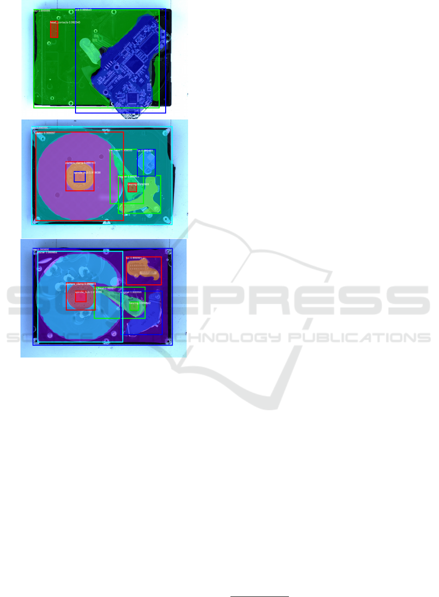
Figure 7: Output of the part segmentation module powered
by MobV1-RCNN on damaged devices, as well as on de-
vices where a part is arbitrarily placed over the device to
create possible occlusion to account for failed manipulation
cases.
posed new part detection and gap detection methods
by using and training state-of-the-art deep learning
networks. We showed on the use-case of a HDD that
the pipeline can achieve a high detection and local-
ization performance, enabling a robot to interact with
the device with sufficient precision. The overall pro-
cess still make some errors (80% AP for screw de-
tection, 24% error for gap detection) but we do not
see this as a limitation: such performance given the
variability of brands, models and state of the device
is acceptable; the goal of this pipeline is to be used in
a more complex system were perception inaccuracies
are handled based on action outcome. To the best of
our knowledge, this is the first approach to provide an
adaptable visual method to analyse a whole device –
in contrast to most of the related work, which focuses
on detecting specific parts or properties of the mate-
rial. This scheme is designed to provide robots with
robust analysis capabilities and open new grounds for
automated disassembly and recycling of End-Of-Life
electronic devices.
One challenge of applying vision methods with
off-the-shelf cameras to such a domain lies in the
presence of shiny and reflective parts. These reduce
the quality of the point-cloud introducing potential er-
rors in the position estimation and the gap detection.
Our system nevertheless provides a relevant analysis
of the hard drive state but the lighting conditions are
a potential failure parameter and should thus be con-
trolled. On the other hand, the method is weakly af-
fected by damages to the device in this use case.
The current need for top-view inputs of the device
limits the ability of the system to analyse all potential
scenes. It can however be overcome by training with
more varied data including side views of the device
(for the part detection and screw detection modules).
For the gap detection, the methods relies on a per-
ceived depth difference so the gaps can be detected
in any position of the device (but are easier to detect
when they are aligned with the stereo camera).
Gap detection can directly be adapted to a new de-
vice as it requires no training data and can be uni-
versally found in any device. The screws used here
are only of Torx8 type and different types of screws
should be included into the training dataset if a dif-
ferent device is to be disassembled. However, this is
not a time consuming task, thanks to the convenient
data collection mode of the screw detector (Yildiz and
Wörgötter, 2019). The part recognition is the least
directly generalizable component and requires collec-
tion, annotation and retraining for other class of de-
vices. However, the HDD use case offers a wide
range of parts that can also be found in other devices
(e.g. PCB, lid and covers), even if they have different
appearances. We will evaluate to which extend the
current system performs well on a set of new devices
in future work.
ACKNOWLEDGMENTS
The research leading to these results has received
funding from the European Union’s Horizon 2020 re-
search and innovation programme under grant agree-
ment no. 731761, IMAGINE. We would like to also
express our gratitude to Maik Bergamos and Electro-
cycling GmbH
4
for the data and hardware used in this
work as well as their expertise on the recycling do-
main.
4
http://www.electrocycling.de
A Visual Intelligence Scheme for Hard Drive Disassembly in Automated Recycling Routines
25

REFERENCES
Abadi, M., Barham, P., Chen, J., Chen, Z., Davis, A.,
Dean, J., Devin, M., Ghemawat, S., Irving, G., Isard,
M., et al. (2016). Tensorflow: A system for large-
scale machine learning. In 12th {USENIX} Sympo-
sium on Operating Systems Design and Implementa-
tion ({OSDI} 16), pages 265–283.
Badrinarayanan, V., Kendall, A., and Cipolla, R. (2017).
Segnet: A deep convolutional encoder-decoder ar-
chitecture for image segmentation. IEEE transac-
tions on pattern analysis and machine intelligence,
39(12):2481–2495.
Bailey-Van Kuren, M. (2002). Automated demanufacturing
studies in detecting and destroying, threaded connec-
tions for processing electronic waste. In Conference
Record 2002 IEEE International Symposium on Elec-
tronics and the Environment (Cat. No.02CH37273),
pages 295–298.
Bdiwi, M., Rashid, A., and Putz, M. (2016). Au-
tonomous disassembly of electric vehicle motors
based on robot cognition. Proceedings - IEEE In-
ternational Conference on Robotics and Automation,
2016-June(July):2500–2505.
Bi, Z. and Wang, L. (2010). Advances in 3d data acquisition
and processing for industrial applications. Robotics
and Computer-Integrated Manufacturing, 26(5):403 –
413.
Bisong, E. (2019). Google colaboratory. In Building Ma-
chine Learning and Deep Learning Models on Google
Cloud Platform, pages 59–64. Springer.
Cai, Z. and Vasconcelos, N. (2018). Cascade r-cnn: Delving
into high quality object detection. In Proceedings of
the IEEE conference on computer vision and pattern
recognition, pages 6154–6162.
Chen, C., Ma, L., Jia, Y., and Zuo, P. (2019). Kidney and
tumor segmentation using modified 3d mask rcnn.
Chollet, F. (2017). Xception: Deep learning with depthwise
separable convolutions. In Proceedings of the IEEE
conference on computer vision and pattern recogni-
tion, pages 1251–1258.
Couteaux, V., Si-Mohamed, S., Nempont, O., Lefevre, T.,
Popoff, A., Pizaine, G., Villain, N., Bloch, I., Cotten,
A., and Boussel, L. (2019). Automatic knee menis-
cus tear detection and orientation classification with
mask-rcnn. Diagnostic and interventional imaging,
100(4):235–242.
Dai, J., He, K., and Sun, J. (2015). Boxsup: Exploiting
bounding boxes to supervise convolutional networks
for semantic segmentation. In 2015 IEEE Interna-
tional Conference on Computer Vision, ICCV 2015,
Santiago, Chile, December 7-13, 2015, pages 1635–
1643. IEEE Computer Society.
Dai, J., He, K., and Sun, J. (2016). Instance-aware semantic
segmentation via multi-task network cascades. In Pro-
ceedings of the IEEE Conference on Computer Vision
and Pattern Recognition, pages 3150–3158.
Duda, R. O. and Hart, P. E. (1971). Use of the hough trans-
formation to detect lines and curves in pictures. Tech-
nical report, SRI Iinternational Menlo Park CA Artifi-
cial Intelligence Center.
Duflou, J. R., Seliger, G., Kara, S., Umeda, Y., Ometto,
A., and Willems, B. (2008). Efficiency and feasibility
of product disassembly: A case-based study. CIRP
Annals, 57(2):583–600.
Dvornik, N., Shmelkov, K., Mairal, J., and Schmid, C.
(2017). Blitznet: A real-time deep network for scene
understanding. In Proceedings of the IEEE interna-
tional conference on computer vision, pages 4154–
4162.
Elsayed, A., Kongar, E., Gupta, S. M., and Sobh, T. (2012).
A robotic-driven disassembly sequence generator for
end-of-life electronic products. Journal of Intelli-
gent and Robotic Systems: Theory and Applications,
68(1):43–52.
Fu, C.-Y., Shvets, M., and Berg, A. C. (2019). Retina-
mask: Learning to predict masks improves state-of-
the-art single-shot detection for free. arXiv preprint
arXiv:1901.03353.
Ghiasi, G. and Fowlkes, C. C. (2016). Laplacian pyramid
reconstruction and refinement for semantic segmenta-
tion. In European Conference on Computer Vision,
pages 519–534. Springer.
Girshick, R. (2015). Fast r-cnn. In Proceedings of the IEEE
international conference on computer vision, pages
1440–1448.
Girshick, R., Donahue, J., Darrell, T., and Malik, J. (2014).
Rich feature hierarchies for accurate object detec-
tion and semantic segmentation. In Proceedings of
the IEEE conference on computer vision and pattern
recognition, pages 580–587.
He, K., Gkioxari, G., Dollár, P., and Girshick, R. (2017).
Mask r-cnn. In Proceedings of the IEEE international
conference on computer vision, pages 2961–2969.
Howard, A. G., Zhu, M., Chen, B., Kalenichenko, D.,
Wang, W., Weyand, T., Andreetto, M., and Adam,
H. (2017). Mobilenets: Efficient convolutional neu-
ral networks for mobile vision applications. arXiv
preprint arXiv:1704.04861.
Huang, G., Liu, Z., and Weinberger, K. Q. (2016).
Densely connected convolutional networks. CoRR,
abs/1608.06993.
Jahanian, A., Le, Q. H., Youcef-Toumi, K., and Tset-
serukou, D. (2019). See the e-waste! training visual
intelligence to see dense circuit boards for recycling.
In Proceedings of the IEEE Conference on Computer
Vision and Pattern Recognition Workshops, pages 0–
0.
Johnson, J. W. (2018). Adapting mask-rcnn for au-
tomatic nucleus segmentation. arXiv preprint
arXiv:1805.00500.
Joulin, A., van der Maaten, L., Jabri, A., and Vasilache, N.
(2016). Learning visual features from large weakly
supervised data. In Computer Vision – ECCV 2016,
pages 67–84.
Karlsson, B. and Järrhed, J.-O. (2000). Recycling of elec-
trical motors by automatic disassembly. Measurement
Science and Technology, 11(4):350–357.
Khoreva, A., Benenson, R., Hosang, J., Hein, M., and
Schiele, B. (2017). Simple does it: Weakly supervised
instance and semantic segmentation. In 2017 IEEE
Conference on Computer Vision and Pattern Recogni-
tion (CVPR), pages 1665–1674.
ROBOVIS 2020 - International Conference on Robotics, Computer Vision and Intelligent Systems
26

Krizhevsky, A., Sutskever, I., and Hinton, G. E. (2012). Im-
agenet classification with deep convolutional neural
networks. In Advances in neural information process-
ing systems, pages 1097–1105.
Li, Y., Qi, H., Dai, J., Ji, X., and Wei, Y. (2017). Fully
convolutional instance-aware semantic segmentation.
In Proceedings of the IEEE Conference on Computer
Vision and Pattern Recognition, pages 2359–2367.
Lin, D., Shen, D., Shen, S., Ji, Y., Lischinski, D., Cohen-
Or, D., and Huang, H. (2019). Zigzagnet: Fusing top-
down and bottom-up context for object segmentation.
In Proceedings of the IEEE Conference on Computer
Vision and Pattern Recognition, pages 7490–7499.
Lin, G., Milan, A., Shen, C., and Reid, I. (2017a). Re-
finenet: Multi-path refinement networks for high-
resolution semantic segmentation. In Proceedings of
the IEEE conference on computer vision and pattern
recognition, pages 1925–1934.
Lin, T.-Y., Dollár, P., Girshick, R., He, K., Hariharan, B.,
and Belongie, S. (2017b). Feature pyramid networks
for object detection. In Proceedings of the IEEE Con-
ference on Computer Vision and Pattern Recognition,
pages 2117–2125.
Lin, T.-Y., Maire, M., Belongie, S., Hays, J., Perona, P.,
Ramanan, D., Dollár, P., and Zitnick, C. L. (2014).
Microsoft coco: Common objects in context. In Euro-
pean conference on computer vision, pages 740–755.
Springer.
Liu, S., Qi, L., Qin, H., Shi, J., and Jia, J. (2018). Path ag-
gregation network for instance segmentation. In Pro-
ceedings of the IEEE Conference on Computer Vision
and Pattern Recognition, pages 8759–8768.
Liu, Y., Wang, Y., Wang, S., Liang, T., Zhao, Q., Tang, Z.,
and Ling, H. (2019). Cbnet: A novel composite back-
bone network architecture for object detection. arXiv
preprint arXiv:1909.03625.
Long, J., Shelhamer, E., and Darrell, T. (2015). Fully con-
volutional networks for semantic segmentation. In
Proceedings of the IEEE conference on computer vi-
sion and pattern recognition, pages 3431–3440.
Malamas, E. N., Petrakis, E. G., Zervakis, M., Petit, L., and
Legat, J.-D. (2003). A survey on industrial vision sys-
tems, applications and tools. Image and Vision Com-
puting, 21(2):171 – 188.
Massari, S. and Ruberti, M. (2013). Rare earth elements as
critical raw materials: Focus on international markets
and future strategies. Resources Policy, 38(1):36–43.
Otsu, N. (1979). A threshold selection method from gray-
level histograms. IEEE transactions on systems, man,
and cybernetics, 9(1):62–66.
Pinheiro, P. O., Lin, T.-Y., Collobert, R., and Dollár, P.
(2016). Learning to refine object segments. In Eu-
ropean Conference on Computer Vision, pages 75–91.
Springer.
Pomares, J., Puente, S., Torres, F., Candelas, F., and Gil,
P. (2004). Virtual disassembly of products based on
geometric models. Computers in Industry, 55(1):1–
14.
Ren, S., He, K., Girshick, R., and Sun, J. (2015). Faster
r-cnn: Towards real-time object detection with region
proposal networks. In Advances in neural information
processing systems, pages 91–99.
Ronneberger, O., Fischer, P., and Brox, T. (2015). U-net:
Convolutional networks for biomedical image seg-
mentation. In International Conference on Medical
image computing and computer-assisted intervention,
pages 234–241. Springer.
Rusu, R. B., Marton, Z. C., Blodow, N., Dolha, M., and
Beetz, M. (2008). Towards 3D Point Cloud Based
Object Maps for Household Environments. Robotics
and Autonomous Systems Journal (Special Issue on
Semantic Knowledge in Robotics), 56(11):927–941.
Sandler, M., Howard, A., Zhu, M., Zhmoginov, A., and
Chen, L.-C. (2018). Mobilenetv2: Inverted residu-
als and linear bottlenecks. In Proceedings of the IEEE
conference on computer vision and pattern recogni-
tion, pages 4510–4520.
Szegedy, C., Vanhoucke, V., Ioffe, S., Shlens, J., and Wo-
jna, Z. (2016). Rethinking the inception architecture
for computer vision. In Proceedings of the IEEE con-
ference on computer vision and pattern recognition,
pages 2818–2826.
Tabuchi, H. (2010). Japan recycles minerals from used elec-
tronics. New York Times, 4.
Tonko, M. and Nagel, H.-H. (2000). Model-based stereo-
tracking of non-polyhedral objects for automatic dis-
assembly experiments. International Journal of Com-
puter Vision, 37(1):99–118.
Torres, F., Puente, S., and Aracil, R. (2003). Disassembly
planning based on precedence relations among assem-
blies. International Journal of Advanced Manufactur-
ing Technology, 21.
Ukida, H. (2007). Visual defect inspection of rotating screw
heads. In SICE Annual Conference 2007, pages 1478–
1483. IEEE.
Wegener, K., Chen, W. H., Dietrich, F., Dröder, K., and
Kara, S. (2015). Robot assisted disassembly for the
recycling of electric vehicle batteries. Procedia CIRP,
29:716–721.
Weigl-Seitz, A., Hohm, K., Seitz, M., and Tolle, H. (2006).
On strategies and solutions for automated disassem-
bly of electronic devices. International Journal of Ad-
vanced Manufacturing Technology, 30(5-6):561–573.
Xie, S., Girshick, R., Dollár, P., Tu, Z., and He, K. (2017).
Aggregated residual transformations for deep neural
networks. In Proceedings of the IEEE conference on
computer vision and pattern recognition, pages 1492–
1500.
Xie, S. Q., Cheng, D., Wong, S., and Haemmerle, E. (2008).
Three-dimensional object recognition system for en-
hancing the intelligence of a KUKA robot. Interna-
tional Journal of Advanced Manufacturing Technol-
ogy, 38(7-8):822–839.
Yildiz, E. and Wörgötter, F. (2019). DCNN-Based
Screw Detection for Automated Disassembly Pro-
cesses. Proceedings of the 15th International Con-
ference on Signal Image Technology & Internet based
Systems.
Zhang, M., Zhou, Y., Zhao, J., Man, Y., Liu, B., and Yao, R.
(2019). A survey of semi- and weakly supervised se-
mantic segmentation of images. Artificial Intelligence
Review.
A Visual Intelligence Scheme for Hard Drive Disassembly in Automated Recycling Routines
27
