
Lane-changing Decision-making using Single-step Deep Q Networ
k
Yizhou Song
1, a
, Kaisheng Huang
1, b, *
and Wei Zhong
1, 2, c
1
The Joint Laboratory for Internet of Vehicles, Ministry of Education - China Mobile Communications Corporation, State
Key Laboratory of Automotive Safety and Energy, School of Vehicle and Mobility, Tsinghua University, Beijing 100084,
China
2
China North Vehicle Institute, Science and Technology on Vehicle Transmission Laboratory, Beijing 100072, China
Keywords: Autonomous Vehicle; Lane-changing Decision-making; Reinforcement Learning.
Abstract: The lane-changing decision-making is a great challenge in autonomous driving system, especially to judge
the feasibility of lane-changing due to the randomness and complexity of surrounding traffic participants.
Reinforcement learning has been shown to outperform many rule-based algorithm for some complex systems.
In this paper, the single-step deep Q network algorithm is proposed by combining single-step reinforcement
learning and deep Q network, and it is applied to judge the feasibility of lane-changing for autonomous
vehicle. In a real-world-like and random traffic environment built in Carmaker, the trained agent can make
correct judgment about the feasibility of lane-changing. Comparing the single-step deep Q network with the
general deep Q network, although the general deep Q network can converge, there are still collisions, and the
agent trained by single-step deep Q network is absolutely safe.
1 INTRODUCTION
The data shows that in the transportation system, 90%
of the total number of traffic accidents are caused by
driver improper operations (Aufrère, R, et.al, 2003).
Autonomous vehicles are developed to eliminate
driver errors to improve traffic safety. Typically, an
autonomous vehicle consists of a perception module,
a decision-making module and a control module (Li,
D, et.al, 2018). The decision-making module makes
correct decisions based on the information of sensors
of the perception module. Making correct decision is
challenging because of the influence of surrounding
traffic participants. The lane-changing decision is
particularly important because collision is more likely
to happen when changing lane compared with driving
in a single lane. In recent years, the lane-changing
decision has gradually become one of the research
focuses in the field of autonomous vehicles.
The methods of lane-changing decision of
autonomous vehicle can be divided into two
categories: rule-based and machine learning-based.
Currently, rule-based methods have been widely
used. And machine learning-based methods have also
proven to perform better in many scenarios in recent
years.
The main method of the rule-based lane change
decision system is the finite state machine method.
This method requires determining multiple states that
an autonomous vehicle may execute, and then
determining the switching conditions between the
states (Schwarting, W, et.al, 2018). Representative
works of this method are the ‘Stanley’ developed by
Stanford University Thrun, S., et.al, 2006) and the
‘Boss’ developed by Carnegie Mellon University
(Urmson, C, et.al, 2008). They decide to execute a
lane-change decision based on some pre-set rules and
thresholds. However, the rule-based method relies too
much on the experience of engineers, and the pre-set
states and thresholds have poor adaptability to
complex traffic conditions. The developers of
‘Junior’ from Stanford University acknowledged that
although the junior was able to complete the DARPA
Challenge, it was unable to cope with real urban
traffic (Chen, J, et.al, 2014).
In recent years, machine learning-based methods
have become the focus of research in the field of
decision-making. Researchers from NVIDIA
(Bojarski, M, et.al, 2016), Intel (Codevilla, F., et.al,
2018) and Comma.ai (Santana, E., & Hotz, G, 2016)
used an end-to-end supervised learning approach to
train decision-making systems for autonomous
vehicles. They used a car equipped with various
Song, Y., Huang, K. and Zhong, W.
Lane-changing Decision-making using Single-step Deep Q Network.
DOI: 10.5220/0010009600250032
In Proceedings of the International Symposium on Frontiers of Intelligent Transport System (FITS 2020), pages 25-32
ISBN: 978-989-758-465-7
Copyright
c
2020 by SCITEPRESS – Science and Technology Publications, Lda. All rights reserved
25

sensors to collect data from all on-board sensors when
the driver was driving the car. By training a
convolutional neural network, the mapping of the
camera's original image to the vehicle control
parameters is completed. This method has a certain
ability to adapt to complex traffic, but it requires a
large amount of data collected in advance, which is
difficult to manipulate in practice.
In addition to end-to-end supervised learning,
reinforcement learning is also widely used in
decision-making systems for autonomous vehicles.
Reinforcement learning is an algorithm that teaches
an agent so that it can perform correct actions in a
random environment to get the maximum reward.
Different from supervised learning, there is no fixed
label for reinforcement learning. Trial and error
methods are used to simulate the learning process. It
is usually implemented in the fields of robot control
(Gu, S., et.al, 2017), autonomous driving (Alizadeh,
A., et.al, 2019), and gaming (Kamaldinov, I., &
Makarov, 2019).
Desjardins et al. (Desjardins, C., & Chaib-Draa, B,
2011) used reinforcement learning to study adaptive
cruise control system. They used policy gradient
reinforcement learning to teach autonomous vehicle
to follow the car in front. Ure et al. (Ure, N. K, 2019)
introduced reinforcement learning based on the
model predictive control adaptive cruise control
system. Reinforcement learning is used to train model
predictive control weights so that autonomous
vehicles can perform better when facing more
complex scenarios.
This paper introduces a single-step deep Q
network algorithm. This algorithm combines single-
step reinforcement learning with deep Q network
algorithm. And it is used to train an autonomous
vehicle to judge the feasibility of lane-change. In this
way, the autonomous vehicle can make correct
decision under different conditions, and ensure the
safety of the lane-changing process.
2 REINFORCEMENT LEARNING
2.1 Deep Reinforcement Learning
In reinforcement learning, agent performs action
according to a policy π. There are two ways to
represent a policy. The first is expressed in the form
of a function aπ
s
, which is a mapping of state
space S to action space A. The second is expressed in
the form of probability π
s,a
, so that
∑
π
s,a
1. In this paper, the policy is expressed as a function.
The quality of a policy can be evaluated using a
state-action value function Q
s,a
. The state-action
value function is defined as the expected value of the
cumulative reward from state s
to state s
, when
perform an action a
at the state s
and keep
interacting with the environment according to the
policy π, i.e.,
Q
s,a
E
R
|s
s,a
a
(1)
R
in (1) is the cumulative reward, and can be
calculated as follows:
R
∑
γ
r
(2)
Where r
is the reward obtained by performing
the action a
in state s
, and γ is the discount factor.
Combining (1) and (2):
Q
s,a
E
∑
γ
r
|s
s,a
a
(3)
The basis of reinforcement learning is the Markov
Decision Process (MDP), which means, the future
state
,…,
of the agent is only related to the
current state s
, and not to the past state
,…,
.
Therefore, the Bellman equation of the state action
value function can be derived by combining (3), i.e.,
Q
s,a
∑
P
R
γQ
s
,a′
(4)
Where P
is the state transition probability, R
is the reward obtained when action a is taken and the
state transfers from s to s
. And a
π
s′
.
The purpose of reinforcement learning is to obtain
the optimum policy π
∗
to maximize the cumulative
reward obtained by the agent, i.e.,
Q
∗
s,a
max
Q
s,a
(5)
Combining (4) and (5) can get the optimal
Bellman equation, i.e.,
Q
∗
s,a
∑
P
R
γmax
Q
∗
s′,a′
(6)
Reinforcement learning to find the optimal policy
is to find the only solution for (6). Traditional
reinforcement learning methods, such as Q learning,
build a Q table to find the optimal solution. The
columns of the Q table represent all states in the state
space, and the rows represent all actions in the action
space. The values in the table are Q values and they
are updated according to (7).
FITS 2020 - International Symposium on Frontiers of Intelligent Transport System
26
Q
s,a
←Q
s,a
α
rγmax
Q
s
,a′
Q
s,a
(7)
Where α is learning rate.
This method has very good results when solving
simple problems. But when the problem becomes
more complicated, especially when the state variable
is continuous, the curse of dimensionality will occur.
Deep Q Network (DQN) can solve the above
problems well. DQN combines deep learning and
reinforcement learning. It utilizes a neural network to
get approximate Q values. Since the neural network
can fit any function, DQN can successfully
approximate the Q value, even if the state space is
multidimensional and continuous.
The input of the neural network in DQN is state,
and the output is the Q value of different actions. At
each training step, DQN saves the current state s
,
action a
, reward r
and next state s
to the replay
memory, and samples a mini-batch of tuples
s
,a
,r
,s
to train the neural network. The
parameter of neural network θ is updated to minimize
the loss function (8).
L
∑
r
γmax
Q
s
,a
Q
s
,a
(8)
θ
is the parameter of target neural network,
which has the same structure as θ, but is updated
more slowly than θ.
2.2
K-armed Bandit Problem
K-armed bandit problem is a single-step
reinforcement learning task, which maximizes the
single-step reward. It is a mathematical model
extracted from the scene of a multi-arm gambling
machine in a casino. The k-armed bandit has k arms.
After placing a coin, a gambler can choose to press
one of the arms. Each arm spit out coins with a certain
probability. The goal is to maximize the reward
through a certain policy, that is, to get the most coins.
Similar to general reinforcement learning
problem, the state-action value function is used to
evaluate the quality of the policy. Since the K-armed
bandit problem is a one-step reinforcement learning
problem, the state of each execution is the same, and
only the action is different, so it can be simplified into
an action value function Q
a
. Q
a
represents the
expected reward obtained after executing action a.
And after the n-th attempt of action a, Q
a
is updated
as:
Q
a
n1
Q
a
r
(9)
3 SCENE STATEMENT
The driver's decision to change lane usually consists
of three steps: making a lane-changing plan, judging
the feasibility of lane-changing, and executing lane-
changing (Hidas, P, 2005). In this paper, we focus on
the step of judging the feasibility of lane-changing.
Generally speaking, the lane-changing plan is made
by the higher-level path-planning module. It may be
a free lane-changing due to obstacles ahead or a
forced lane-changing to reach the destination. In this
paper, we use a random number to simulate the lane-
changing plan made by the driver. An LQR-based
path tracking method is used to execute lane-
changing with the goal of minimizing distance and
deviation angle to the path at previewed point.
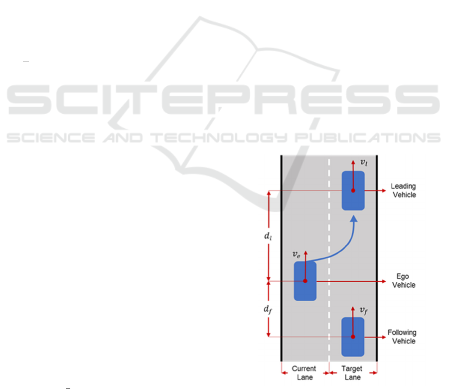
The research scenario of this paper is shown in
Fig. 1. The autonomous vehicle expects to change
from the current lane to the target lane, and there may
be a leading vehicle and a following vehicle on the
target lane.
v
, v
and v
are velocity of ego vehicle, leading
vehicle and following vehicle respectively. d
is the
distance between the ego vehicle and the leading
vehicle, and d
is the distance between the ego
vehicle and the following vehicle.
This paper aims to use reinforcement learning to
teach autonomous vehicle to judge if it is proper to
change lane, with the goal to start lane-changing as
early as possible to improve traffic efficiency and
avoid collisions during lane-changing.
Figure 1: Lane-Changing Scenario.
Lane-changing Decision-making using Single-step Deep Q Network
27

4 METHODOLOGY
In this section, how to train agent is described. The
reinforcement learning model and the dynamic traffic
environment are explained in detail.
4.1 Reinforcement Learning Model
We consider the process of an autonomous vehicle
making a lane-changing decision as MDP. The
autonomous vehicle is the agent which needs to be
trained. The environment includes lanes, the
conditions of the ego vehicle and vehicles in the target
lane.
As described in Fig. 1, when the autonomous
vehicle makes a lane-changing decision, the main
basis is the condition of the ego vehicle and the
condition of the ego vehicle relative to the vehicles in
the target lane. So we took the absolute velocity of the
ego vehicle v
, the relative velocity between the ego
vehicle and the obstacle vehicle ∆v
v
v
, and
the relative distance d
as the state representations. i
represents l or f, that is, leading vehicle or following
vehicle. If there is no vehicle in the position of leading
vehicle or following vehicle, the relative distance d
is set to the maximum distance of the sensor which is
200 m, and the relative velocity ∆v
is set to 0. The
state vector consists of five continuous variables:
s
v
,d
,∆v
,d
,∆v
(10)
Generally, there are two actions that can be
selected for autonomous vehicle: lane-changing or no
lane-changing. In this paper, when the autonomous
vehicle makes a lane-changing decision, the order
cannot be withdrawn, which means the lane-changing
decision must be the last step of each training episode.
In addition, since the reward obtained by the agent
after a decision of not changing lane is a fixed value,
then an output of the neural network is also a fixed
value, which does not make sense. Therefore, when
training the agent, this paper only studies the last step
of each training episode, that is, the step where the
agent makes a lane-changing decision. In other
words, there is only one action of the reinforcement
learning model:
a: change lane.
The reward function is defined as follows:
r
1, successfullanechanging
5, collision
(11)
The problem studied in this paper is a maximal
single-step reward reinforcement learning problem
which is similar to the "K-armed Bandit Problem".
Since there is only one action, the state-action value
function is expressed as follows:
Q
s
E
r
|s
s
(12)
Where Q
s
represents the expected reward
obtained when the lane-changing decision is
performed in state s. It can be written as below:
Q
s
p
s
r
p
s
r
s.t. p
s
p
s
1
(13)
Where p
s
and p
s
are the probability of
successful lane-changing and collision after
executing lane-changing in state s, respectively; r
and r
are the reward for successful lane-changing
and collision, respectively. According to (11), r
1
and r
5.
The state variables are continuous values, so a
neural network will be used to represent Q
s
combined with deep reinforcement learning. The
parameters of the neural network were updated to
minimize the loss function:
L
∑
r
Q
s
(14)
Although only one action is set when establishing
a reinforcement learning model, it does not mean that
the autonomous vehicle can only execute lane-
changing action. Autonomous vehicle will execute
the action based on the value of Q
s
. In this paper,
as shown in (11), a successful lane-changing gets a
positive reward while a failed lane-changing gets a
negative reward, so the reward for not changing lane
is set to a constant 0, which can be considered as the
state-action value function that does not execute lane-
changing. Therefore, the autonomous vehicle will
choose whether to execute lane-changing based on
Q
s
:
Q
s
0: change lane, and
Q
s
0: not change lane.
4.2 Environment
In this paper, CarMaker developed by IPG
Automotive GmbH is utilized as the simulator to
build the traffic environment for training the
autonomous vehicle. Compared to general traffic
simulators, CarMaker is more focused on the vehicle
itself, and has a better vehicle dynamics model. An
illustration of CarMaker is shown in Fig. 2.
FITS 2020 - International Symposium on Frontiers of Intelligent Transport System
28
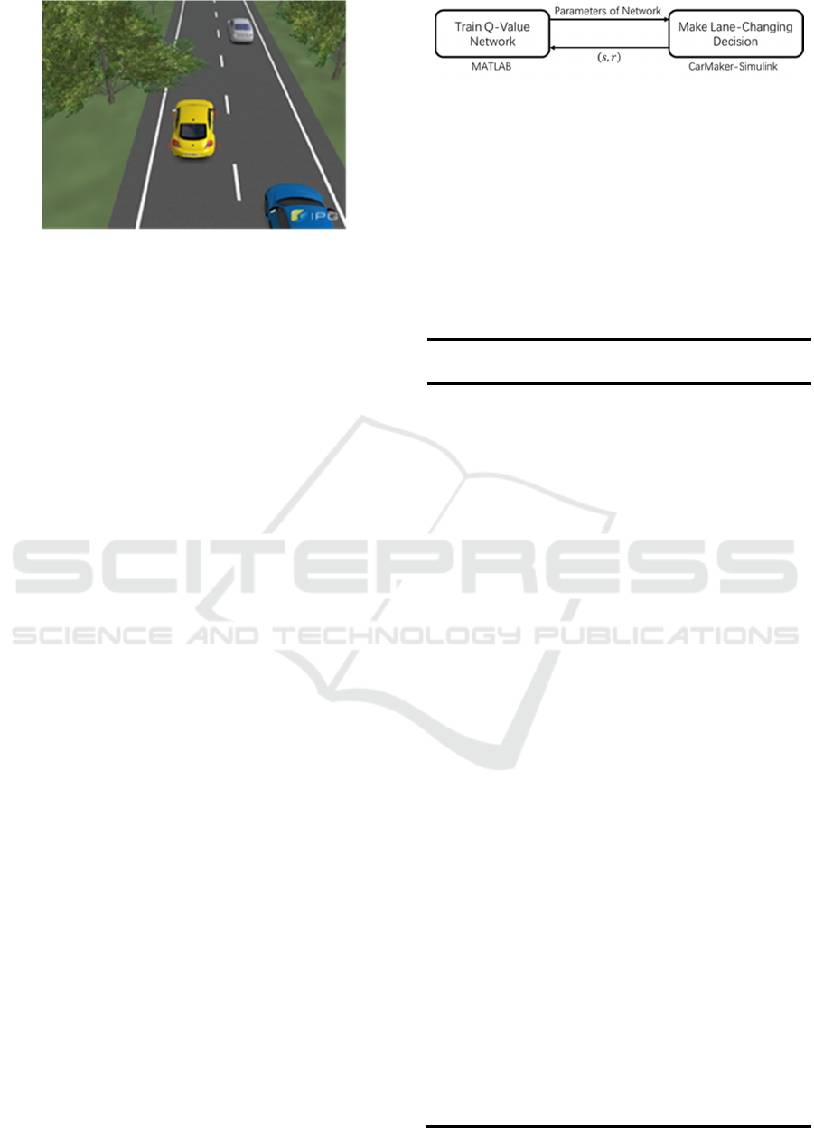
Figure 2: Screenshot of CarMaker.
A one-way road with two lanes is built in
CarMaker as shown in Fig. 2. The yellow vehicle in
the left lane is the autonomous vehicle studied in this
paper. Its behaviour is controlled by our algorithm.
There are several vehicles in the right lane. Their
behaviours are controlled by both our settings and the
IPG Driver model set by CarMaker. They run at
random speeds according to our settings, but at the
same time they meet the restrictions of the IPG Driver
model. The minimum distance between them is
d
t
vd
, where t
1.5s is the
headway time, d
3m is the static distance to the
front vehicle. All data of all vehicles, including
vehicle speed and longitudinal position, can be
provided directly by CarMaker.
5 TRAINING AND RESULT
5.1
Training Setup
In this paper, MATLAB is utilized to build and train
the neural network, which is the Q value network.
During the training process, the interaction between
MATLAB and CarMaker-Simulink is shown in Fig.
3.
While training the agent, there is a balance
between exploration and exploitation. If the agent
chooses to explore only, then all the trial
opportunities are evenly distributed to each state, and
eventually the expected Q value of each state can be
obtained, but obviously the training time is very long.
On the other hand, if the agent chooses to exploit
only, each time it only executes the action with the
highest Q value. The training time is short, but it is
difficult to get the global optimal solution.
Figure 3: Interaction between MATLAB and CarMaker-
Simulink.
ε-greedy algorithm is used to solve the problem of
exploration and exploitation. The agent explores with
a probability of ε and exploits with a probability of
1ε
. When ε0, the optimal action is chosen,
and when ε1, the agent chooses the action
completely randomly. In this paper, instead of being
a constant, ε will gradually decrease with training as
below:
Algorithm 1: Single-Step DQN for Lane-
Changing.
Initialize replay memory D with infinite capacity
Initialize state value function Q with random
weights θ
for episode1,M do
Initialize action a: not change lane
while a: not change lane do
Read the state s from CarMaker
Initialize a random number rnd∈
0,1
if tt
then
if rndε then
Randomly select action a: change lane or not
change lane
else
if Q
s
0 then
a: change lane
else
a: not change lane
end if
end if
end if
end while
Start lane-changing
if collision then
r5
else
r1
end if
Store transition
s,r
in D
if episodeN
then
Sample random mini-batch of transitions
s
,r
from D
Perform a gradient descent step on r
Q
s
with respect to θ
end if
end for
Lane-changing Decision-making using Single-step Deep Q Network
29
ε
ε
ε
e
ε
(15)
In the simulator, the speeds of all vehicles,
including the ego-vehicle and traffic vehicles, change
randomly and constantly. During the lane-changing
process, the speed of the ego-vehicle will be constant,
and the speeds of traffic vehicles are changing all the
time to simulate the unknown behaviour of the
surrounding vehicles in actual traffic.
In addition, to ensure the randomness of the initial
conditions, we set a random start time t
∈
0,50
s. The training starts when the simulation time
is bigger than t
,. This can be understood as the
higher-level path-planning module making a lane-
changing plan at t
.
During training, in order to ensure that the agent
has enough experience, we set a threshold for the
number of replay memory N
, and training will
only start when the number of replay memory is
greater than N
.
The details of the single-step DQN algorithm used
in this paper for the lane-changing decision are shown
in Algorithm 1.
The algorithm consists of three steps. The first
step is to determine whether a lane-changing decision
could be made before making a lane-changing
decision. The second step is that after the agent has
made a lane-changing decision, the agent begins to
change lane. The third step is to store the data in the
replay memory after the lane-changing is completed
(there may be a successful lane-changing or a
collision), and train the agent with the data in the
replay memory.
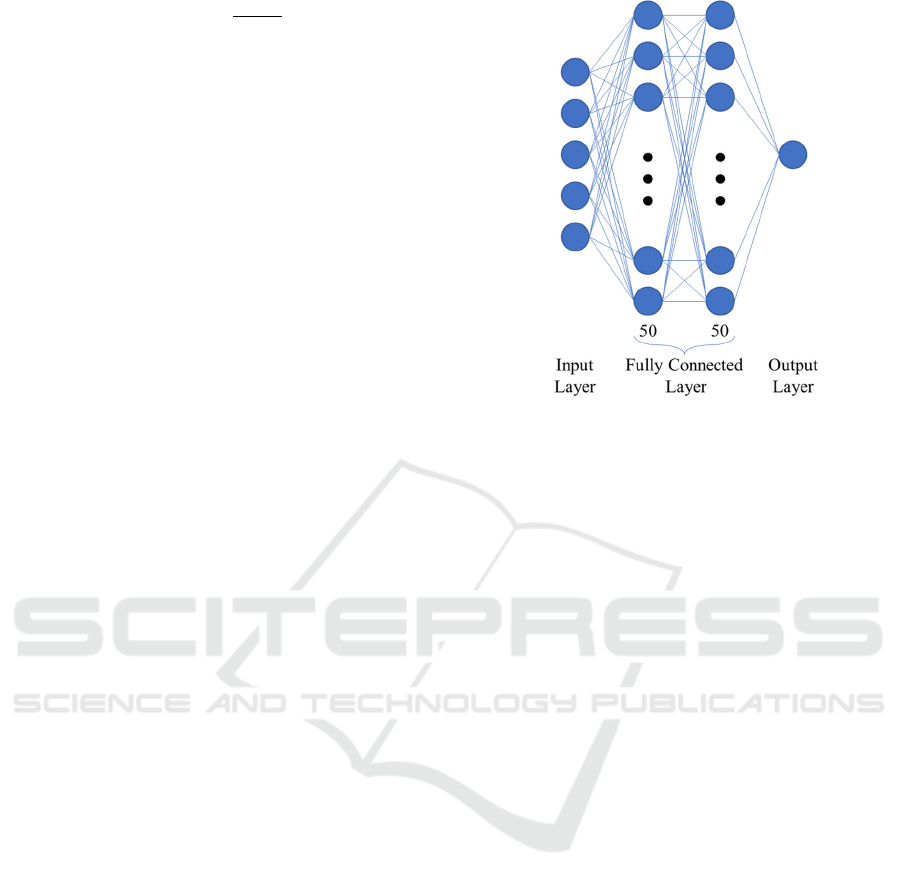
5.2
Training Configurations
A neural network with the structure shown in Fig. 4
is used to approximate the Q value function. It
consists of two fully connected layers, each
consisting of 50 nodes. The input is the state, and the
output is the Q value for executing the action in that
state, that is, the expected reward obtained by
executing a lane-changing in the given state. The tanh
function is selected as the hidden layer activation
function.
Figure 4: Structure of the Neural Network.
The maximum training episodes M was set to
6,000. The threshold of the replay memory at the
beginning of training N
is 200, that is, the training
does not start until the agent has completed 200
explorations. The Adam optimizer is selected to
update neural network parameters with a learning rate
of 0.001 and the mini-batch of 32. For ε-greedy
algorithm, we set ε
0.9, ε
0 and
ε
200.
5.3
Results
Since the initial state of each training episode is
completely random, it is very likely that there is no
obstacle vehicle in the target lane when the
autonomous vehicle starts to make lane-changing
decision, so the result of a single training episode
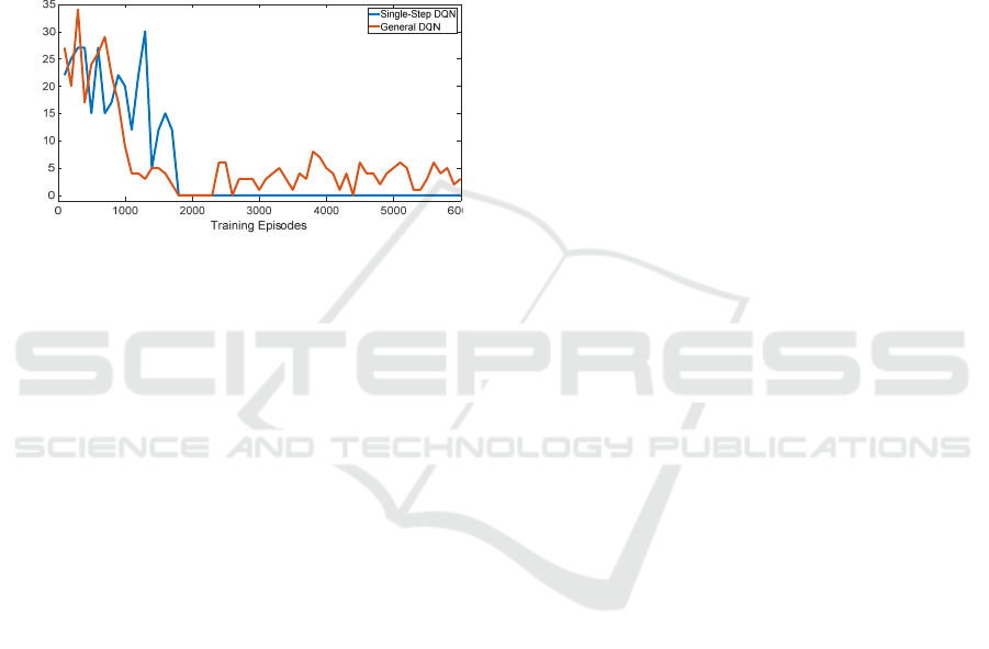
cannot be used to evaluate the algorithm. In this
paper, we use the number of collisions of the
autonomous vehicle per 100 training episodes to
evaluate the result. The result is shown in Fig. 5.
In addition, a general DQN method is used to
solve the same problem as a comparison. The general
DQN uses two actions, that is, the Q network has two
outputs, one is the Q value for executing lane-
changing, and the other is the Q value for not
executing lane-changing. The reward is set as (16).
The discount factor is 0.99. The replay memory
capacity is 10,000. The frequency of updating the
target Q network is 2,000. The result is also shown in
Fig. 5.
FITS 2020 - International Symposium on Frontiers of Intelligent Transport System
30
r
1, successfullanechanging
5, collision
0, notexecutelanechanging
(16)
As shown in Fig. 5, the numbers of collisions for
single-step DQN and general DQN both decrease
during training. After 1,700 training episodes, there is
no more collisions happening for single-step DQN.
But general DQN cannot completely converge to 0.
This shows that our algorithm can converge better. It
can teach the autonomous vehicle to learn to judge the
feasibility of lane-changing ensuring absolute safety.
Figure 5: Training Results.
6 CONCLUSIONS
In this paper, we proposed a new method to judge the
feasibility when the autonomous vehicle is going to
change the lane. The method combines the single-step
reinforcement learning and the deep reinforcement
learning. We use the single-step reinforcement
learning framework that learns by solving the
expected reward for executing different actions in the
same state. Aiming at the problem of discontinuous
states or actions in this framework, combined with the
idea of DQN, a neural network is used to approximate
the Q value function. The proposed single-step DQN
algorithm judges the feasibility of lane-changing
based on the lane-changing plan made by the high-
layer path planning module and the surrounding
vehicle state obtained by sensors. The instruction is
sent to the low-level control module, which uses the
LQR-based method to complete the lane-changing.
The final results indicate that the proposed method in
this paper can ensure that the lane-changing process
of autonomous vehicle is absolutely safe.
ACKNOWLEDGEMENTS
This work was supported by the European Union’s
Horizon 2020 research and innovation programme
under the Marie Skłodowska-Curie grant agreement
No 824019, and Beijing Municipal Science and
Technology Commission under Grant
D17110000491701.
REFERENCES
Alizadeh, A., Moghadam, M., Bicer, Y., et al. Automated
Lane Change Decision Making using Deep
Reinforcement Learning in Dynamic and Uncertain
Highway Environment. 2019 IEEE Intelligent
Transportation Systems Conference (ITSC). October,
2019. pp. 1399-1404.
Aufrère, R., Gowdy, J., Mertz, C., et al. Perception for
collision avoidance and autonomous driving.
Mechatronics, 13.10 (2003), 1149-1161.
Bojarski, M., Del Testa, D., Dworakowski, D., et al. End to
end learning for self-driving cars. (2016). arXiv
preprint arXiv:1604.07316.
Chen, J., Zhao, P., Liang, H., et al. A multiple attribute-
based decision making model for autonomous vehicle
in urban environment. 2014 IEEE Intelligent Vehicles
Symposium Proceedings. June, 2014. pp. 480-485.
Codevilla, F., Miiller, M., López, A., et al. End-to-end
driving via conditional imitation learning. 2018 IEEE
International Conference on Robotics and Automation
(ICRA). May, 2018. pp. 1-9.
Desjardins, C., & Chaib-Draa, B. Cooperative adaptive
cruise control: A reinforcement learning approach.
IEEE Transactions on intelligent transportation
systems, (2011) 12(4), 1248-1260.
Gu, S., Holly, E., Lillicrap, T., et al. Deep reinforcement
learning for robotic manipulation with asynchronous
off-policy updates. 2017 IEEE international conference
on robotics and automation (ICRA). May, 2017. pp.
3389-3396.
Hidas, P. Modelling vehicle interactions in microscopic
simulation of merging and weaving. Transportation
Research Part C: Emerging Technologies. (2005) 13(1),
37-62.
Kamaldinov, I., & Makarov, I. Deep reinforcement learning
in match-3 game. 2019 IEEE conference on games
(CoG). August, 2019. pp. 1-4.
Li, D., Zhao, D., Zhang, Q., et al. Reinforcement learning
and deep learning based lateral control for autonomous
driving. (2018). arXiv preprint arXiv:1810.12778.
Santana, E., & Hotz, G. Learning a driving simulator.
(2016). arXiv preprint arXiv:1608.01230.
Schwarting, W., Alonso-Mora, J., & Rus, D. Planning and
decision-making for autonomous vehicles. Annual
Review of Control, Robotics, and Autonomous
Systems. (2018).
Collision Numbers
per 100 Episodes
Lane-changing Decision-making using Single-step Deep Q Network
31

Thrun, S., Montemerlo, M., Dahlkamp, H., et al. Stanley:
The robot that won the DARPA Grand Challenge.
Journal of field Robotics, (2006) 23(9), 661-692.
Ure, N. K., Yavas, M. U., Alizadeh, A., et al. Enhancing
situational awareness and performance of adaptive
cruise control through model predictive control and
deep reinforcement learning. 2019 IEEE Intelligent
Vehicles Symposium (IV). June, 2019. pp. 626-631.
Urmson, C., Anhalt, J., Bagnell, D., et al. Autonomous
driving in urban environments: Boss and the urban
challenge. Journal of Field Robotics, (2008) 25(8), 425-
466.
FITS 2020 - International Symposium on Frontiers of Intelligent Transport System
32
